Hexo

vectorbt学习_45DMA之五滑窗网格参数优选

Posted on 2024-06-28 Edited on 2026-03-11 In 06重拾量化 , btvt

本文在上一篇文章(05dma_03rollingGridParamV2)面临问题
对于双均线，最终采用参数为(20，22),(30，35)这样的参数组合，显然不合理，有对行情进行拟合的嫌疑。
较合理的参数组合方式是，采用快线以及慢线相对快线的倍率。大致认为剔除二者相关性了（正交性）。
此时就无法借助run_combs创建组合计算指标了，需基于vbt创建新技术指标DualMA。

勘误：此篇文章部分截图可能有误，此文章的后继文章“DMA之六滑窗网格参数优选”修复此问题。请查阅后文。

01,基础配置信息

#conda envs:vectorbt_env
import warnings
import vectorbt as vbt
import numpy as np
import pandas as pd
from datetime import datetime, timedelta
import pytz
from dateutil.parser import parse
import ipywidgets as widgets
from copy import deepcopy
from tqdm import tqdm
import imageio
from IPython import display
import plotly.graph_objects as go
import itertools
import dateparser
import gc
import math
from tools import dbtools 

warnings.filterwarnings("ignore")

pd.set_option('display.max_rows',500)
pd.set_option('display.max_columns',500)
pd.set_option('display.width',1000)

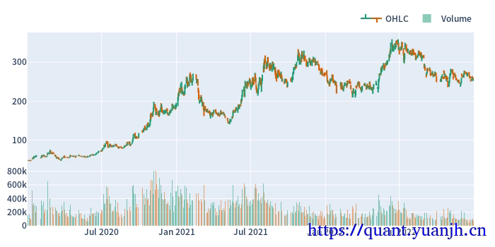
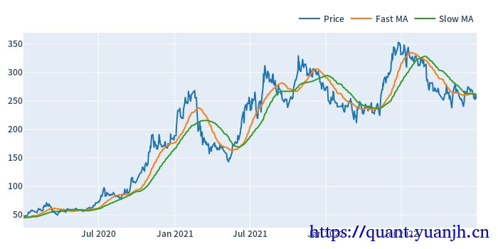
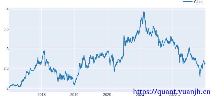
02,行情获取和可视化

a,时间交易参数配置

# Enter your parameters here
seed = 42
symbol = '002594.XSHE'
metric = 'total_return'

start_date = datetime(2020, 1, 1, tzinfo=pytz.utc)  # time period for analysis, must be timezone-aware
end_date = datetime(2023,1,1, tzinfo=pytz.utc)
time_buffer = timedelta(days=100)  # buffer before to pre-calculate SMA/EMA, best to set to max window
freq = '1D'

vbt.settings.portfolio['init_cash'] = 10000.  # 100$
vbt.settings.portfolio['fees'] = 0.0025  # 0.25%
vbt.settings.portfolio['slippage'] = 0.0025  # 0.25%

b,获取行情和行情mask

# Download data with time buffer
cols = ['Open', 'High', 'Low', 'Close', 'Volume']
# ohlcv_wbuf = vbt.YFData.download(symbol, start=start_date-time_buffer, end=end_date).get(cols)

ohlcv_wbuf=dbtools.MySQLData.download(symbol).get() # 自带工具类查询
assert(~ohlcv_wbuf.empty)
ohlcv_wbuf = ohlcv_wbuf.astype(np.float64)

print("ohlcv_wbuf.shape:",ohlcv_wbuf.shape)
print("ohlcv_wbuf.columns:",ohlcv_wbuf.columns)


# Create a copy of data without time buffer
wobuf_mask = (ohlcv_wbuf.index >= start_date) & (ohlcv_wbuf.index <= end_date) # mask without buffer

ohlcv = ohlcv_wbuf.loc[wobuf_mask, :]

print("ohlcv.shape:",ohlcv.shape)

# Plot the OHLC data
ohlcv.vbt.ohlcv.plot().show_svg() # 绘制蜡烛图
# remove show_svg() to display interactive chart!

ohlcv_wbuf.shape: (978, 5)
ohlcv_wbuf.columns: Index(['Open', 'High', 'Low', 'Close', 'Volume'], dtype='object')
ohlcv.shape: (728, 5)

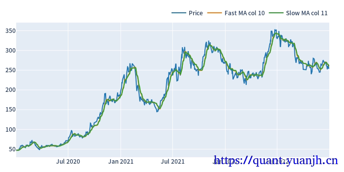
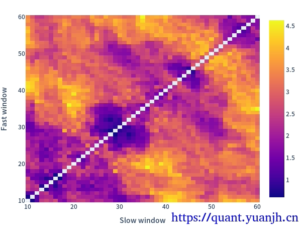
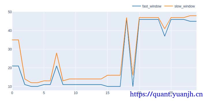
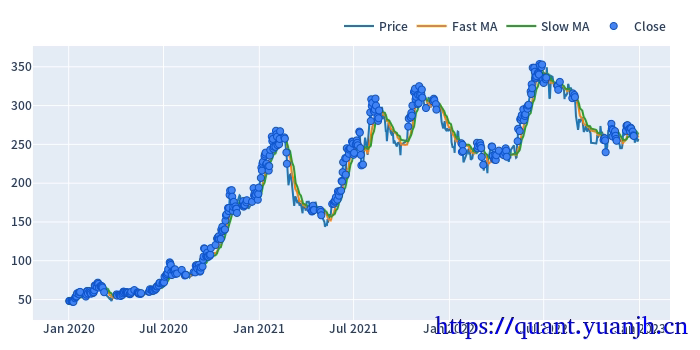
20,网格参数-指标计算和可视化

仅可视化第一列

fast_windows = np.arange(10, 50,5)
slow_multis = np.arange(1.5, 5.5, 0.5)
print("fast_windows:",fast_windows)
print("slow_multis:",slow_multis)

price=ohlcv_wbuf['Close']
dualma = vbt.DualMA.run(price, fast_window=fast_windows,slow_multi=slow_multis,param_product=True)
dualma = dualma[wobuf_mask]
# there should be no nans after removing time buffer
assert(~dualma.fast_ma.isnull().any().any())
assert(~dualma.slow_ma.isnull().any().any())


print()
print('dualma.fast_ma.head(3)')
print(dualma.fast_ma.head(3))
print('dualma.slow_ma.head(3)')
print(dualma.slow_ma.head(3))

print()
fig = ohlcv['Close'].vbt.plot(trace_kwargs=dict(name='Price'))
fig = dualma.fast_ma.iloc[:,0].vbt.plot(trace_kwargs=dict(name="Fast MA col %s"%str(dualma.fast_ma.iloc[:,0].name)), fig=fig)
fig = dualma.slow_ma.iloc[:,0].vbt.plot(trace_kwargs=dict(name="Slow MA col %s"%str(dualma.slow_ma.iloc[:,0].name)), fig=fig)
fig.show_svg()

fast_windows: [10 15 20 25 30 35 40 45]
slow_multis: [1.5 2.  2.5 3.  3.5 4.  4.5 5. ]

dualma.fast_ma.head(3)
dualma_fast_window             10                                                                 15                                                                                    20                                                                      25                                                                        30                                                                                      35                                                                                    40                                                                        45                                                                             
dualma_slow_multi             1.5     2.0     2.5     3.0     3.5     4.0     4.5     5.0        1.5        2.0        2.5        3.0        3.5        4.0        4.5        5.0      1.5      2.0      2.5      3.0      3.5      4.0      4.5      5.0      1.5      2.0      2.5      3.0      3.5      4.0      4.5      5.0        1.5        2.0        2.5        3.0        3.5        4.0        4.5        5.0        1.5        2.0        2.5        3.0        3.5        4.0        4.5        5.0      1.5      2.0      2.5      3.0      3.5      4.0      4.5      5.0        1.5        2.0        2.5        3.0        3.5        4.0        4.5        5.0
date                                                                                                                                                                                                                                                                                                                                                                                                                                                                                                                                                                                                                                                                             
2020-01-02 00:00:00+00:00  46.665  46.665  46.665  46.665  46.665  46.665  46.665  46.665  45.824667  45.824667  45.824667  45.824667  45.824667  45.824667  45.824667  45.824667  45.3025  45.3025  45.3025  45.3025  45.3025  45.3025  45.3025  45.3025  44.9476  44.9476  44.9476  44.9476  44.9476  44.9476  44.9476  44.9476  44.816667  44.816667  44.816667  44.816667  44.816667  44.816667  44.816667  44.816667  44.594571  44.594571  44.594571  44.594571  44.594571  44.594571  44.594571  44.594571  44.5425  44.5425  44.5425  44.5425  44.5425  44.5425  44.5425  44.5425  44.440222  44.440222  44.440222  44.440222  44.440222  44.440222  44.440222  44.440222
2020-01-03 00:00:00+00:00  46.972  46.972  46.972  46.972  46.972  46.972  46.972  46.972  46.128667  46.128667  46.128667  46.128667  46.128667  46.128667  46.128667  46.128667  45.5025  45.5025  45.5025  45.5025  45.5025  45.5025  45.5025  45.5025  45.1420  45.1420  45.1420  45.1420  45.1420  45.1420  45.1420  45.1420  44.964000  44.964000  44.964000  44.964000  44.964000  44.964000  44.964000  44.964000  44.723714  44.723714  44.723714  44.723714  44.723714  44.723714  44.723714  44.723714  44.6265  44.6265  44.6265  44.6265  44.6265  44.6265  44.6265  44.6265  44.555556  44.555556  44.555556  44.555556  44.555556  44.555556  44.555556  44.555556
2020-01-06 00:00:00+00:00  47.138  47.138  47.138  47.138  47.138  47.138  47.138  47.138  46.456000  46.456000  46.456000  46.456000  46.456000  46.456000  46.456000  46.456000  45.7310  45.7310  45.7310  45.7310  45.7310  45.7310  45.7310  45.7310  45.3376  45.3376  45.3376  45.3376  45.3376  45.3376  45.3376  45.3376  45.112667  45.112667  45.112667  45.112667  45.112667  45.112667  45.112667  45.112667  44.871143  44.871143  44.871143  44.871143  44.871143  44.871143  44.871143  44.871143  44.7115  44.7115  44.7115  44.7115  44.7115  44.7115  44.7115  44.7115  44.660222  44.660222  44.660222  44.660222  44.660222  44.660222  44.660222  44.660222
dualma.slow_ma.head(3)
dualma_fast_window                10                                                                              15                                                                                      20                                                                                25                                                                                 30                                                                                    35                                                                                      40                                                                                   45                                                                             
dualma_slow_multi                1.5      2.0      2.5        3.0        3.5      4.0        4.5      5.0        1.5        2.0        2.5        3.0        3.5        4.0        4.5        5.0        1.5      2.0      2.5        3.0        3.5        4.0        4.5      5.0        1.5      2.0        2.5        3.0        3.5      4.0        4.5       5.0        1.5        2.0        2.5        3.0        3.5        4.0        4.5      5.0        1.5        2.0        2.5        3.0        3.5        4.0        4.5        5.0        1.5        2.0      2.5        3.0        3.5        4.0        4.5       5.0        1.5        2.0        2.5        3.0        3.5        4.0        4.5        5.0
date                                                                                                                                                                                                                                                                                                                                                                                                                                                                                                                                                                                                                                                                                                                             
2020-01-02 00:00:00+00:00  45.824667  45.3025  44.9476  44.816667  44.594571  44.5425  44.440222  44.6384  45.180455  44.816667  44.545676  44.440222  44.717692  45.135167  45.513134  46.025200  44.816667  44.5425  44.6384  45.135167  45.697429  46.307750  46.683111  47.0983  44.545676  44.6384  45.235806  46.025200  46.560460  47.0983  47.997679  48.61136  44.440222  45.135167  46.025200  46.683111  47.425238  48.410917  48.769630  48.8484  44.717692  45.697429  46.560460  47.425238  48.496066  48.803714  48.852357  49.430914  45.135167  46.307750  47.0983  48.410917  48.803714  48.892313  49.622778  50.14240  45.513134  46.683111  47.997679  48.769630  48.852357  49.622778  50.162574  50.375822
2020-01-03 00:00:00+00:00  46.128667  45.5025  45.1420  44.964000  44.723714  44.6265  44.555556  44.6660  45.373636  44.964000  44.652162  44.555556  44.741538  45.119167  45.485821  45.984267  44.964000  44.6265  44.6660  45.119167  45.666714  46.291125  46.643333  47.0707  44.652162  44.6660  45.229677  45.984267  46.549080  47.0707  47.936429  48.56848  44.555556  45.119167  45.984267  46.643333  47.349905  48.362083  48.758074  48.8320  44.741538  45.666714  46.549080  47.349905  48.460984  48.784357  48.838471  49.366457  45.119167  46.291125  47.0707  48.362083  48.784357  48.878875  49.584500  50.12260  45.485821  46.643333  47.936429  48.758074  48.838471  49.584500  50.141139  50.379778
2020-01-06 00:00:00+00:00  46.456000  45.7310  45.3376  45.112667  44.871143  44.7115  44.660222  44.6908  45.562273  45.112667  44.787297  44.660222  44.773846  45.116667  45.474478  45.950800  45.112667  44.7115  44.6908  45.116667  45.641143  46.267875  46.621889  47.0449  44.787297  44.6908  45.232742  45.950800  46.534598  47.0449  47.864554  48.52880  44.660222  45.116667  45.950800  46.621889  47.278952  48.320667  48.743185  48.8232  44.773846  45.641143  46.534598  47.278952  48.406803  48.770500  48.833885  49.298743  45.116667  46.267875  47.0449  48.320667  48.770500  48.860063  49.552222  50.09115  45.474478  46.621889  47.864554  48.743185  48.833885  49.552222  50.122772  50.388044

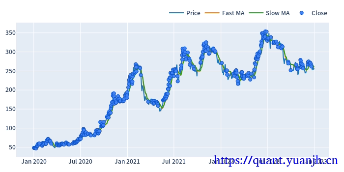
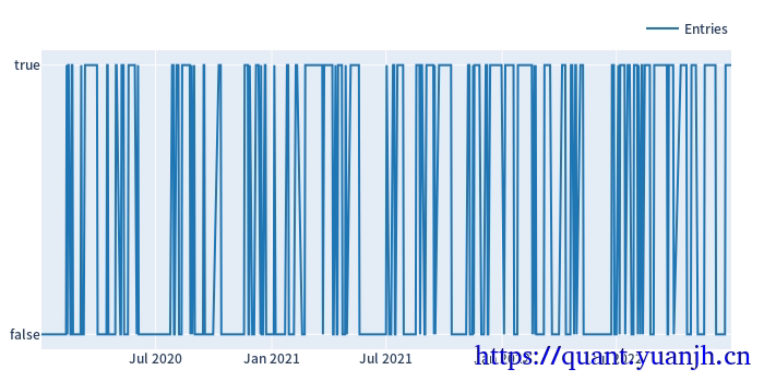
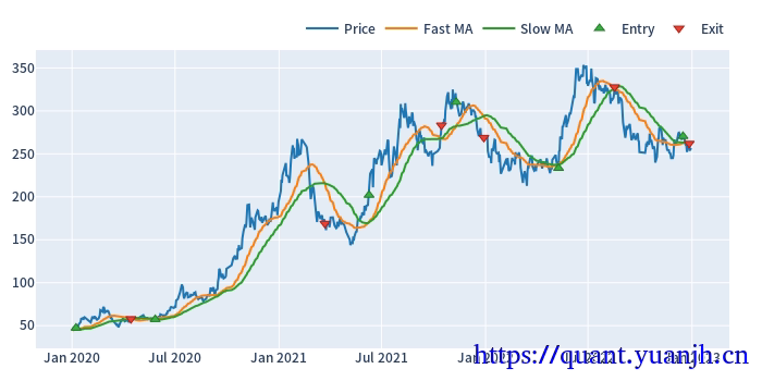
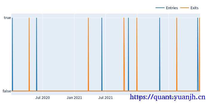
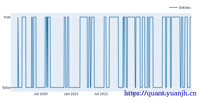
21,网格参数-信号计算和可视化

仅可视化第一列

dmac_size.shape: (728, 64)

dmac_size.iloc[:3,:3]:
dualma_fast_window           10            
dualma_slow_multi           1.5   2.0   2.5
date                                       
2020-01-02 00:00:00+00:00  True  True  True
2020-01-03 00:00:00+00:00  True  True  True
2020-01-06 00:00:00+00:00  True  True  True

Start                       2020-01-02 00:00:00+00:00
End                         2022-12-30 00:00:00+00:00
Period                                            728
Total                                       474.03125
Rate [%]                                    65.114183
First Index                 2020-01-15 16:52:30+00:00
Last Index                  2022-11-07 20:15:00+00:00
Norm Avg Index [-1, 1]                      -0.159967
Distance: Min                                     1.0
Distance: Max                               82.734375
Distance: Mean                               1.464916
Distance: Std                                5.175417
Total Partitions                             6.671875
Partition Rate [%]                           1.510978
Partition Length: Min                       41.671875
Partition Length: Max                      211.171875
Partition Length: Mean                     110.468174
Partition Length: Std                       78.523847
Partition Distance: Min                      26.78125
Partition Distance: Max                     82.734375
Partition Distance: Mean                    51.365493
Partition Distance: Std                     28.015768
Name: agg_func_mean, dtype: object

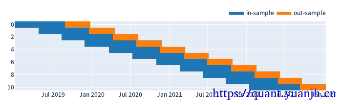
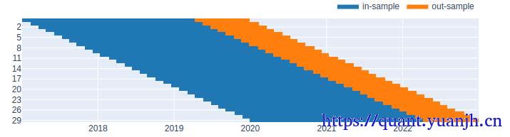
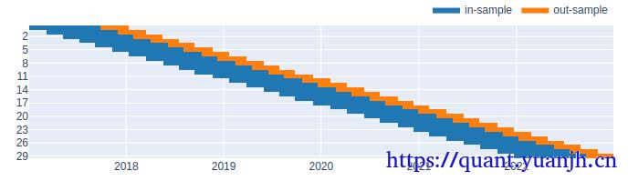
22,行情,信号的滑窗处理

注意点：
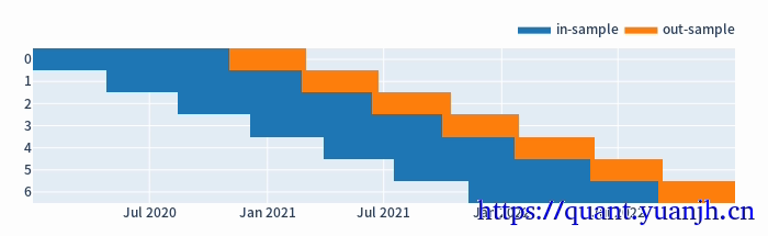
01，训练集和验证集比例3：1，或者2：1，对应：window_len和set_lens为4:1(或3:1)，过大了历史包袱沉重，无法及时响应最新行情，过小了则容易参数跳变，形成类似过拟合效果

a,参数设置和效果预览

代码中

#todo 这里是自然日计算的，但后面训练，验证集个数计算都完全正确，哪里应该和预想的不一致
合理的。实测bar_days= 60时

print(in_indexes[0][0])
print(in_indexes[1][0])
print(in_indexes[0][53:55])

2019-01-02 00:00:00+00:00
2019-03-25 00:00:00+00:00
DatetimeIndex(['2019-03-25 00:00:00+00:00', '2019-03-26 00:00:00+00:00'], dtype='datetime64[ns, UTC]', name='split_0', freq=None)
可见第二行第一个位于第一行第53个，不足设置的60,就是由于切分优先保证了数据的足量，但是数据间隔方面则可能有所重叠。

# 滚动周期参数设置和大致效果可视化
start_end_days=int((end_date-start_date).days) #todo 这里是自然日计算的，但后面训练，验证集个数计算都完全正确，哪里应该和预想的不一致
bar_days= 80         # 训练，验证集时间长度，以此为单位
test_bar_num=2      # 训练集时间长度
verify_bar_num=1    # 验证集时间长度
verify_overlap=0 # 验证集重叠时间长度
pre_test_days=0    # 由于测试集一部分时间用于计算指标，导致实际训练时间不足，这个是一定程度补充的days周期
# n取值需要满足:确保验证集合收尾相接
# => (n-1)*(verify_bar_num-verify_overlap)+(verify_bar_num+test_bar_num)=start_end_days/bar_days
# => n=(start_end_days/bar_days-test_bar_num-verify_overlap)/(verify_bar_num-verify_overlap)
calc_n=(start_end_days/bar_days-test_bar_num-verify_overlap)/(verify_bar_num-verify_overlap)


split_kwargs = dict(
    n=int(calc_n), 
    window_len=int(bar_days*(test_bar_num+verify_bar_num)+pre_test_days), 
    set_lens=(int(bar_days*verify_bar_num),), 
    left_to_right=False
)  # 10 windows, each 2 years long, reserve 180 days for test
# 合理设置n，最好确保验证集，连续且无重复
pf_kwargs = dict(
    direction='both',  # long and short
    freq='d'
)
print('split_kwargs:',split_kwargs)

def roll_in_and_out_samples(price, **kwargs):
    return price.vbt.rolling_split(**kwargs)

# 验证：单列数据验证，橘黄色验证集连续且无重复
roll_in_and_out_samples(price, **split_kwargs, plot=True, trace_names=['in-sample', 'out-sample']).show_svg()

split_kwargs: {'n': 11, 'window_len': 240, 'set_lens': (80,), 'left_to_right': False}

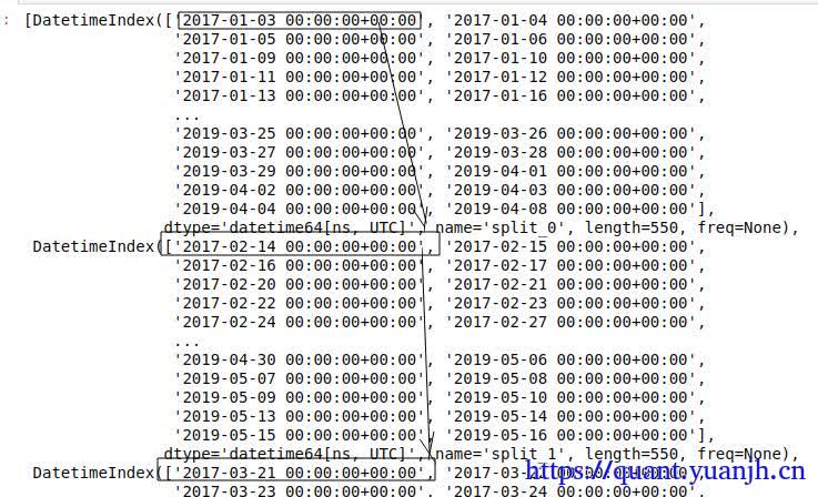
b,根据滑窗参数切分行情数据和信号

in_price.shape: (160, 11)
out_price.shape: (80, 11)

in_price.index: RangeIndex(start=0, stop=160, step=1)
in_price.columns: Int64Index([0, 1, 2, 3, 4, 5, 6, 7, 8, 9, 10], dtype='int64', name='split_idx')

in_price[0:3]:
split_idx     0      1      2      3      4      5       6       7       8       9       10
0          49.17  58.15  51.20  43.39  48.15  97.90  167.98  239.52  202.00  251.77  253.14
1          48.06  56.16  49.50  43.15  49.73  96.55  164.08  225.00  214.11  252.50  266.49
2          50.65  55.36  50.29  43.79  52.25  94.50  168.03  208.99  227.02  246.86  266.08

###############################
in_dmac_size.shape: (160, 704)
out_dmac_size.shape: (80, 704)

in_dmac_size.iloc[:5,:5]:
split_idx              0                        
dualma_fast_window    10                        
dualma_slow_multi    1.5   2.0   2.5   3.0   3.5
0                   True  True  True  True  True
1                   True  True  True  True  True
2                   True  True  True  True  True
3                   True  True  True  True  True
4                   True  True  True  True  True

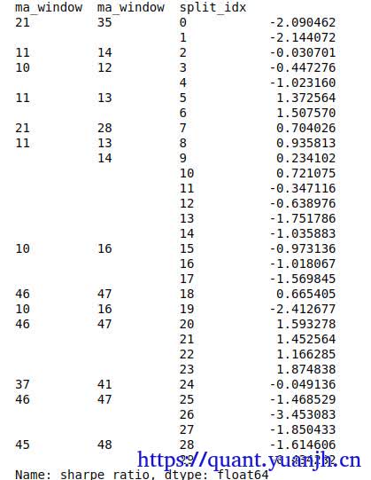
23,滑窗的收益数据计算

a,持有参数收益

在此区间，基础标的物表现


def simulate_holding(price, **kwargs):
    pf = vbt.Portfolio.from_holding(price, **kwargs)
    return pf.sharpe_ratio()

in_hold_sharpe = simulate_holding(in_price, **pf_kwargs)
print(in_hold_sharpe.head(5))

out_hold_sharpe = simulate_holding(out_price, **pf_kwargs)
print(out_hold_sharpe.head(5))

split_idx
0    0.235446
1   -1.630616
2    0.598889
3    2.647397
4    4.501923
Name: sharpe_ratio, dtype: float64
split_idx
0   -0.929956
1    2.065991
2    4.100300
3    4.801291
4    0.688785
Name: sharpe_ratio, dtype: float64

b,网格参数收益(训练集和验证集)

in_sharpe.shape: (704,)
dualma_fast_window  dualma_slow_multi  split_idx
10                  1.5                0            0.235446
                    2.0                0            0.235446
                    2.5                0            0.235446
                    3.0                0            0.235446
                    3.5                0            0.235446
                                                      ...   
45                  3.0                10           0.663486
                    3.5                10           0.663486
                    4.0                10           0.663486
                    4.5                10           0.663486
                    5.0                10           0.663486
Name: sharpe_ratio, Length: 704, dtype: float64

out_sharpe.shape: (704,)
dualma_fast_window  dualma_slow_multi  split_idx
10                  1.5                0           -0.929956
                    2.0                0           -0.820595
                    2.5                0           -0.820595
                    3.0                0           -0.820595
                    3.5                0           -0.820595
                                                      ...   
45                  3.0                10          -0.554763
                    3.5                10          -0.554763
                    4.0                10          -0.554763
                    4.5                10          -0.554763
                    5.0                10          -0.554763
Name: sharpe_ratio, Length: 704, dtype: float64

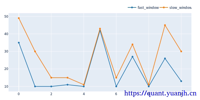
c,训练集上的最佳参数用于验证集

大致思路：
01,获取各split_idx的最佳收益(sharp_radio)的参数组合idxmax,也就是fast_window,slow_window,split_idx，三维索引元组
02,按照split_idx进行聚类，取得各split_idx对应的最佳参数。实际含义就是各滑动窗口的最佳参数

def get_best_index(performance, higher_better=True):
    if higher_better:
        return performance[performance.groupby('split_idx').idxmax()].index
    return performance[performance.groupby('split_idx').idxmin()].index
in_best_index = get_best_index(in_sharpe)

print('in_best_index[:5]')
print(in_best_index[:5])

# 参数走势可视化
def get_best_params(best_index, level_name):
    return best_index.get_level_values(level_name).to_numpy()
in_best_fast_windows = get_best_params(in_best_index, 'dualma_fast_window')
in_best_slow_multi = get_best_params(in_best_index, 'dualma_slow_multi')
in_best_slow_windows = in_best_fast_windows*in_best_slow_multi
in_best_window_pairs = np.array(list(zip(in_best_fast_windows, in_best_slow_windows)))
print()
print('in_best_window_pairs[:5][:]:')
print(in_best_window_pairs[:5][:])
pd.DataFrame(in_best_window_pairs, columns=['fast_window', 'slow_window']).vbt.plot().show_svg()

in_best_index[:5]
MultiIndex([(40, 5.0, 0),
            (10, 3.0, 1),
            (10, 1.5, 2),
            (10, 1.5, 3),
            (10, 1.5, 4)],
           names=['dualma_fast_window', 'dualma_slow_multi', 'split_idx'])

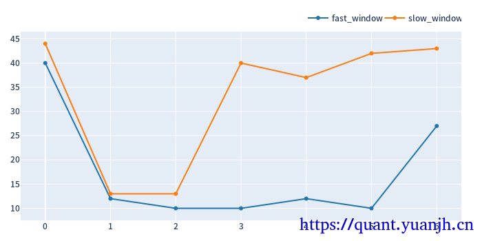
in_best_window_pairs[:5][:]:
[[ 40. 200.]
 [ 10.  30.]
 [ 10.  15.]
 [ 10.  15.]
 [ 10.  15.]]

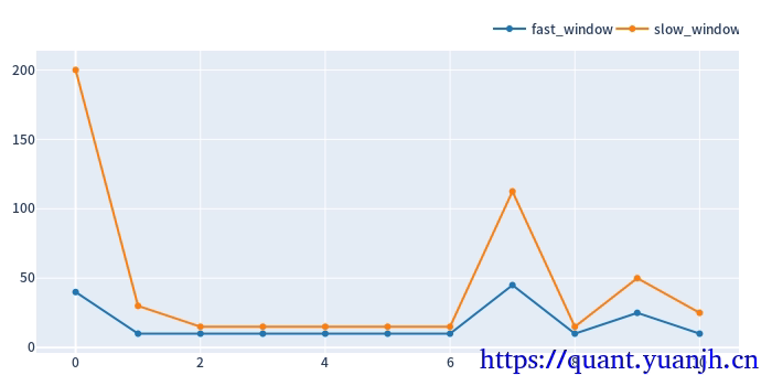
将滚动获取的最佳参数用于验证集，统计收益信息

in_best_index.shape: (11,)

in_best_index:
MultiIndex([(40, 5.0,  0),
            (10, 3.0,  1),
            (10, 1.5,  2),
            (10, 1.5,  3),
            (10, 1.5,  4),
            (10, 1.5,  5),
            (10, 1.5,  6),
            (45, 2.5,  7),
            (10, 1.5,  8),
            (25, 2.0,  9),
            (10, 2.5, 10)],
           names=['dualma_fast_window', 'dualma_slow_multi', 'split_idx'])

out_dmac_size.shape: (80, 704)

out_dmac_size_reindexed[in_best_index].shape: (80, 11)

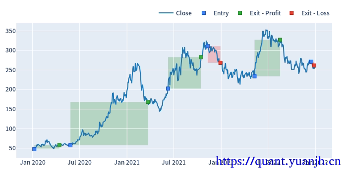
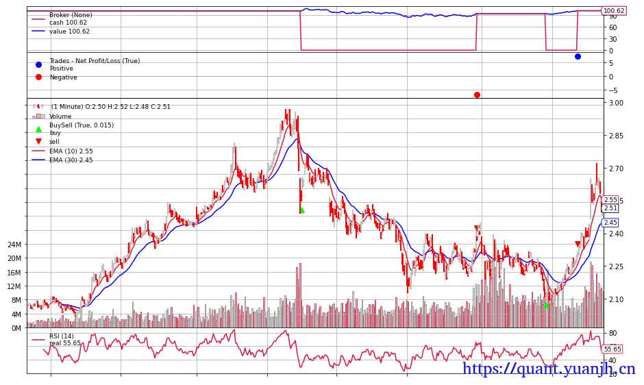
dmac_pf_out.trades.records[:5]
   id  col        size  entry_idx  entry_price  entry_fees  exit_idx  exit_price  exit_fees           pnl    return  direction  status  parent_id
0   0    0  199.762836          0    49.934525   24.937656        79       46.85        0.0   -641.111119 -0.064271          0       0          0
1   1    1  222.599259          0    44.811750   24.937656        79       58.80        0.0   3088.836429  0.309656          0       0          1
2   2    2  182.338041          0    54.706425   24.937656        79       88.73        0.0   6178.854345  0.619430          0       0          2
3   3    3  114.462060          0    87.147325   24.937656        79      183.53        0.0  11007.221874  1.103474          0       0          3
4   4    4   59.581957          0   167.417500   24.937656        79      176.88        0.0    538.856616  0.054020          0       0          4

out_test_sharpe.head(5)
dualma_fast_window  dualma_slow_multi  split_idx
40                  5.0                0           -0.929956
10                  3.0                1            2.065991
                    1.5                2            4.100300
                                       3            4.801291
                                       4            0.688785
Name: sharpe_ratio, dtype: float64

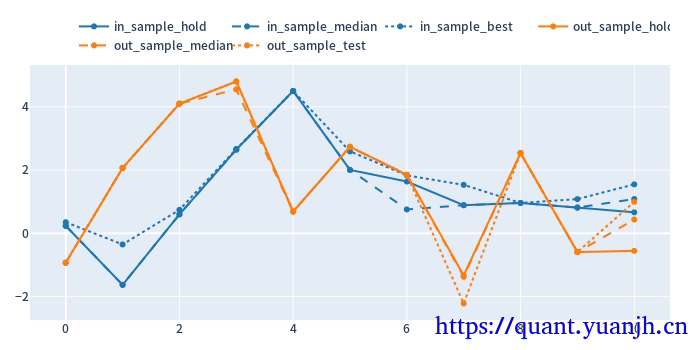
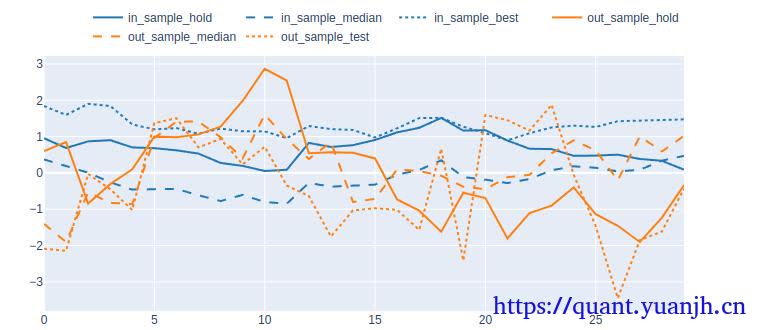
24,sharp ratio的汇总可视化

cv_results_df = pd.DataFrame({
    'in_sample_hold': in_hold_sharpe.values,
    'in_sample_median': in_sharpe.groupby('split_idx').median().values,
    'in_sample_best': in_sharpe[in_best_index].values,
    'out_sample_hold': out_hold_sharpe.values,
    'out_sample_median': out_sharpe.groupby('split_idx').median().values,
    'out_sample_test': out_test_sharpe.values
})

color_schema = vbt.settings['plotting']['color_schema']

cv_results_df.vbt.plot(
    trace_kwargs=[
        dict(line_color=color_schema['blue']),
        dict(line_color=color_schema['blue'], line_dash='dash'),
        dict(line_color=color_schema['blue'], line_dash='dot'),
        dict(line_color=color_schema['orange']),
        dict(line_color=color_schema['orange'], line_dash='dash'),
        dict(line_color=color_schema['orange'], line_dash='dot')
    ]
).show_svg()

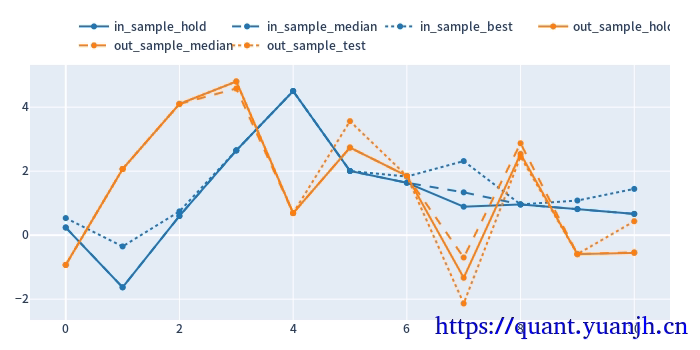
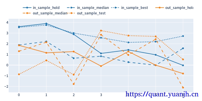
关注点：

蓝色部分
正常排序是(从上到下)：点线，实现，线段，

橘色部分

实线对实线
说明测试集和验证集的周期收益情况，二者同时出现0轴同侧较好（同时上涨，同时下跌，保持行情的稳定性or延续性）

线段对线段
二者一方面随着各自颜色的实线趋势变化（受各自实线影响较大），其他应该无必然联系

点线对点线
蓝色点高于橘色点线，蓝色是训练集内最佳，橘色则是训练集得到最优参数用于验证集结果收益，大概率低于验证集。

测试，验证集时间长度差异，引入偏差
由于测试集一般是验证集的2-3倍（或更多），对于单边行情(假如上涨)，则(测试集的)实线收益。蓝色线大概率位于橘色线上方。
如果下跌，则相反。蓝色由于时间长，大概率位于橘色下方。

注意：
01，202406，对于当前case，y周取值为sharp ratio夏普比，而非收益率。所以数据点高低并不反映收益率。
所以，以上结论需要稍斟酌，并不完全准确。

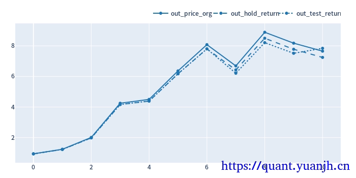
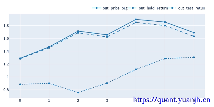
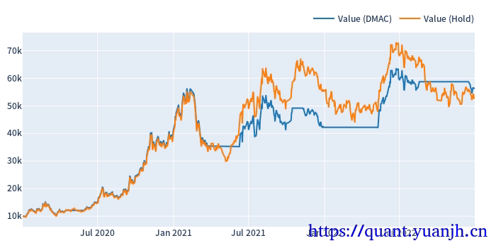
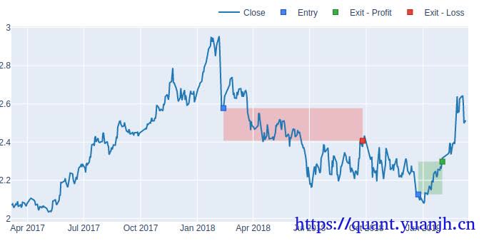
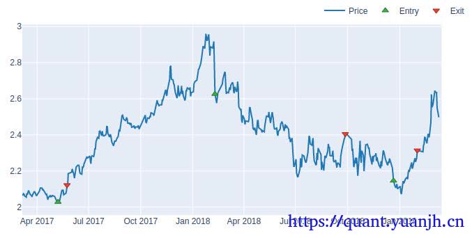
25,滚动回测收益可视化

# 验证集：原始价格变动
out_price_org=out_price.iloc[-1, :]/out_price.iloc[0, :]
print('out_price_org shape:',out_price_org.shape)
print('out_price_org.head(5)')
print(out_price_org.head(5))

# 验证集：持有收益率
def simulate_holding(price, **kwargs):
    pf = vbt.Portfolio.from_holding(price, **kwargs)
    return pf.total_return()

out_hold_return = simulate_holding(out_price, **pf_kwargs)
print()
print('out_hold_return shape:',out_hold_return.shape)
print('out_hold_return.head(5) + 1')
print(out_hold_return.head(5)+1)


print()
print('out_test_return shape:',out_test_return.shape)
print('out_test_return.head(5) + 1')
print(out_test_return.head(5)+1)

cv_results_df = pd.DataFrame({
    'out_price_org':  out_price_org.cumprod(),
    'out_hold_return': (out_hold_return.values+1).cumprod(),
    'out_test_return': (out_test_return.values+1).cumprod()
})

color_dmac_pfschema = vbt.settings['plotting']['color_schema']


cv_results_df.vbt.plot(
    trace_kwargs=[
        dict(line_color=color_schema['blue']),
        dict(line_color=color_schema['blue'], line_dash='dash'),
        dict(line_color=color_schema['blue'], line_dash='dot')
    ]
).show_svg()

out_price_org shape: (11,)
out_price_org.head(5)
split_idx
0    0.940574
1    1.315436
2    1.625985
3    2.111239
4    1.059162
dtype: float64

out_hold_return shape: (11,)
out_hold_return.head(5) + 1
split_idx
0    0.935889
1    1.308884
2    1.617885
3    2.100722
4    1.053886
Name: total_return, dtype: float64

out_test_return shape: (11,)
out_test_return.head(5) + 1
dualma_fast_window  dualma_slow_multi  split_idx
40                  5.0                0            0.935889
10                  3.0                1            1.308884
                    1.5                2            1.617885
                                       3            2.100722
                                       4            1.053886
Name: total_return, dtype: float64

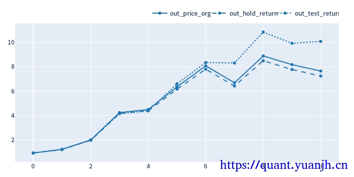
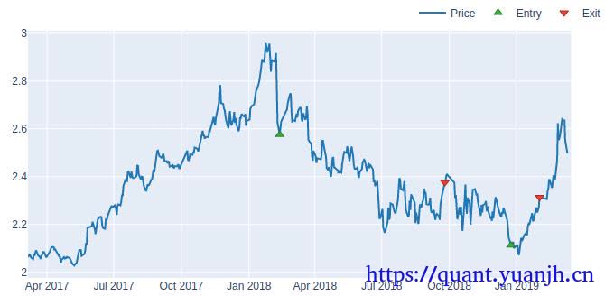
可见，在上次降低技术指标的预热时间优化的基础上，整体收益进一步提升。改进后的策略避免了参数过拟合，挺高了鲁棒性，带来了收益改善。

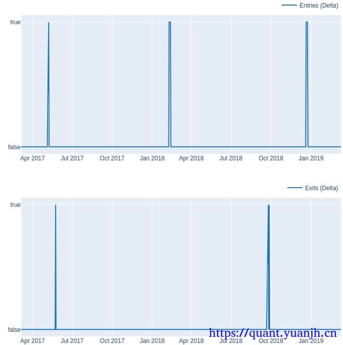
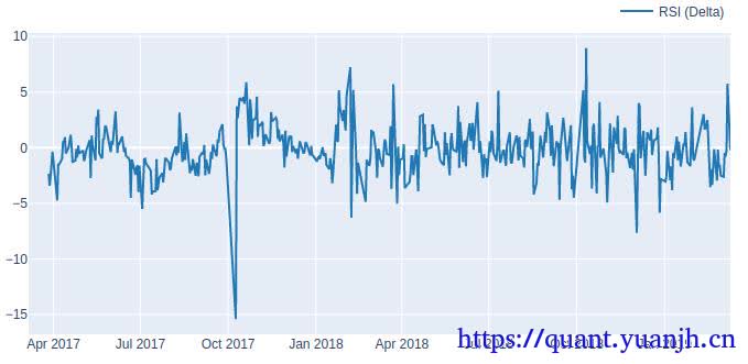
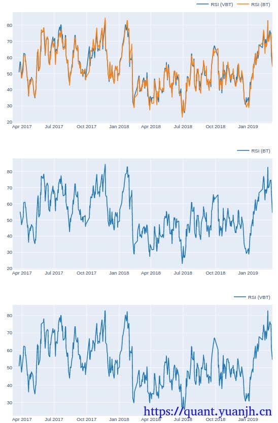
26,计算正确性验证(略)

a,准备校验数据，数据展示
b,行情->指标 计算正确
c,指标->信号 计算正确
d,信号->交易 计算正确

vectorbt学习_44DMA之四滑窗网格参数优选

Posted on 2024-06-28 Edited on 2026-03-11 In 06重拾量化 , btvt

本文在上一篇文章(vectorbt学习_17DMA之三滑窗网格参数优选)面临问题
时间切分后，根据切分后的行情数据，重新计算技术指标，会存在一部分行情作为技术指标的预热时间被消耗掉。
比如：训练集，验证集时间(80,40), slow_windows=30，慢均线需要30天才有有效值。
则意味着训练集需要只有50(80-30)天，预测集10(40-30)天，技术指标slow_ma有有效取值。实际训练，验证集为(50,10)，与本意偏差较大。

勘误：此篇文章部分截图可能有误，此文章的后继文章“DMA之六滑窗网格参数优选”修复此问题。请查阅后文。

01,基础配置信息

#conda envs:vectorbt_env
import warnings
import vectorbt as vbt
import numpy as np
import pandas as pd
from datetime import datetime, timedelta
import pytz
from dateutil.parser import parse
import ipywidgets as widgets
from copy import deepcopy
from tqdm import tqdm
import imageio
from IPython import display
import plotly.graph_objects as go
import itertools
import dateparser
import gc
import math
from tools import dbtools 

warnings.filterwarnings("ignore")

pd.set_option('display.max_rows',500)
pd.set_option('display.max_columns',500)
pd.set_option('display.width',1000)

02,行情获取和可视化

a,时间交易参数配置

# Enter your parameters here
seed = 42
symbol = '002594.XSHE'
metric = 'total_return'

start_date = datetime(2020, 1, 1, tzinfo=pytz.utc)  # time period for analysis, must be timezone-aware
end_date = datetime(2023,1,1, tzinfo=pytz.utc)
time_buffer = timedelta(days=100)  # buffer before to pre-calculate SMA/EMA, best to set to max window
freq = '1D'

vbt.settings.portfolio['init_cash'] = 10000.  # 100$
vbt.settings.portfolio['fees'] = 0.0025  # 0.25%
vbt.settings.portfolio['slippage'] = 0.0025  # 0.25%

b,获取行情和行情mask

# Download data with time buffer
cols = ['Open', 'High', 'Low', 'Close', 'Volume']
# ohlcv_wbuf = vbt.YFData.download(symbol, start=start_date-time_buffer, end=end_date).get(cols)

ohlcv_wbuf=dbtools.MySQLData.download(symbol).get() # 自带工具类查询
assert(~ohlcv_wbuf.empty)
ohlcv_wbuf = ohlcv_wbuf.astype(np.float64)

print("origin ohlcv_wbuf size:",ohlcv_wbuf.shape)
print(ohlcv_wbuf.columns)


# Create a copy of data without time buffer
wobuf_mask = (ohlcv_wbuf.index >= start_date) & (ohlcv_wbuf.index <= end_date) # mask without buffer

ohlcv = ohlcv_wbuf.loc[wobuf_mask, :]

print("wobuf_mask ohlcv size:",ohlcv.shape)

# Plot the OHLC data
ohlcv.vbt.ohlcv.plot().show_svg() # 绘制蜡烛图
# remove show_svg() to display interactive chart!

origin ohlcv_wbuf size: (978, 5)
Index(['Open', 'High', 'Low', 'Close', 'Volume'], dtype='object')
wobuf_mask ohlcv size: (728, 5)

20,网格参数-指标计算和可视化

仅可视化第一列

price=ohlcv_wbuf['Close']
windows = np.arange(10, 50)

fast_ma, slow_ma = vbt.MA.run_combs(price, windows, r=2, short_names=['fast', 'slow'])

print(fast_ma.ma.shape)
print(slow_ma.ma.shape)

# Remove time buffer
fast_ma = fast_ma[wobuf_mask]
slow_ma = slow_ma[wobuf_mask]

# there should be no nans after removing time buffer
assert(~fast_ma.ma.isnull().any().any())
assert(~slow_ma.ma.isnull().any().any())

print(fast_ma.ma.shape)
print(slow_ma.ma.shape)


fig = ohlcv['Close'].vbt.plot(trace_kwargs=dict(name='Price'))
fig = fast_ma.ma.iloc[:,0].vbt.plot(trace_kwargs=dict(name="Fast MA col %d"%fast_ma.ma.iloc[:,0].name), fig=fig)
fig = slow_ma.ma.iloc[:,0].vbt.plot(trace_kwargs=dict(name="Slow MA col %d"%slow_ma.ma.iloc[:,0].name), fig=fig)
fig.show_svg()

(978, 780)
(978, 780)
(728, 780)
(728, 780)

21,网格参数-信号计算和可视化

仅可视化第一列

dmac_size.shape: (728, 780)
dmac_size.iloc[:3,:3]:
fast_window                  10            
slow_window                  11    12    13
date                                       
2020-01-02 00:00:00+00:00  True  True  True
2020-01-03 00:00:00+00:00  True  True  True
2020-01-06 00:00:00+00:00  True  True  True

Start                                 2020-01-02 00:00:00+00:00
End                                   2022-12-30 00:00:00+00:00
Period                                                      728
Total                                                423.078205
Rate [%]                                              58.115138
First Index                           2020-01-02 02:00:00+00:00
Last Index                  2022-12-27 06:59:04.615384576+00:00
Norm Avg Index [-1, 1]                                -0.179136
Distance: Min                                               1.0
Distance: Max                                         75.946154
Distance: Mean                                         1.720602
Distance: Std                                          5.889353
Total Partitions                                      14.607692
Partition Rate [%]                                     3.501842
Partition Length: Min                                  3.239744
Partition Length: Max                                 85.138462
Partition Length: Mean                                36.392118
Partition Length: Std                                 27.476308
Partition Distance: Min                                4.425641
Partition Distance: Max                               75.946154
Partition Distance: Mean                              29.174564
Partition Distance: Std                               26.152924
Name: agg_func_mean, dtype: object

22,行情,信号的滑窗处理

a,参数设置和效果预览

代码中

# todo这里是自然日计算的，但后面训练，验证集个数计算都完全正确，哪里应该和预想的不一致
合理的。实测bar_days= 60时

print(in_indexes[0][0])
print(in_indexes[1][0])
print(in_indexes[0][53:55])

2019-01-02 00:00:00+00:00
2019-03-25 00:00:00+00:00
DatetimeIndex(['2019-03-25 00:00:00+00:00', '2019-03-26 00:00:00+00:00'], dtype='datetime64[ns, UTC]', name='split_0', freq=None)
可见第二行第一个位于第一行第53个，不足设置的60,就是由于切分优先保证了数据的足量，但是数据间隔方面则可能有所重叠。

# 滚动周期参数设置和大致效果可视化
start_end_days=int((end_date-start_date).days) #todo 这里是自然日计算的，但后面训练，验证集个数计算都完全正确，哪里应该和预想的不一致
bar_days= 80         # 训练，验证集时间长度，以此为单位
test_bar_num=2      # 训练集时间长度
verify_bar_num=1    # 验证集时间长度
verify_overlap=0 # 验证集重叠时间长度
pre_test_days=0    # 由于测试集一部分时间用于计算指标，导致实际训练时间不足，这个是一定程度补充的days周期
# n取值需要满足:确保验证集合收尾相接
# => (n-1)*(verify_bar_num-verify_overlap)+(verify_bar_num+test_bar_num)=start_end_days/bar_days
# => n=(start_end_days/bar_days-test_bar_num-verify_overlap)/(verify_bar_num-verify_overlap)
calc_n=(start_end_days/bar_days-test_bar_num-verify_overlap)/(verify_bar_num-verify_overlap)


split_kwargs = dict(
    n=int(calc_n), 
    window_len=int(bar_days*(test_bar_num+verify_bar_num)+pre_test_days), 
    set_lens=(int(bar_days*verify_bar_num),), 
    left_to_right=False
)  # 10 windows, each 2 years long, reserve 180 days for test
# 合理设置n，最好确保验证集，连续且无重复
pf_kwargs = dict(
    direction='both',  # long and short
    freq='d'
)
print('split_kwargs:',split_kwargs)

def roll_in_and_out_samples(price, **kwargs):
    return price.vbt.rolling_split(**kwargs)

# 验证：单列数据验证，橘黄色验证集连续且无重复
roll_in_and_out_samples(price, **split_kwargs, plot=True, trace_names=['in-sample', 'out-sample']).show_svg()

# 大致观察数据特征
(in_price, in_indexes), (out_price, out_indexes) = roll_in_and_out_samples(price, **split_kwargs)

print('in_price.shape:',in_price.shape )  # in-sample
print('out_price.shape:',out_price.shape)
print('in_price.index:',in_price.index)
print('in_price.columns:',in_price.columns)
print('in_price[0:3]:',in_price[0:3])

print('in_indexes[:5]:',in_indexes[:3])

split_kwargs: {'n': 11, 'window_len': 240, 'set_lens': (80,), 'left_to_right': False}

in_price.shape: (160, 11)
out_price.shape: (80, 11)
in_price.index: RangeIndex(start=0, stop=160, step=1)
in_price.columns: Int64Index([0, 1, 2, 3, 4, 5, 6, 7, 8, 9, 10], dtype='int64', name='split_idx')
in_price[0:3]: split_idx     0      1      2      3      4      5       6       7       8       9       10
0          49.17  58.15  51.20  43.39  48.15  97.90  167.98  239.52  202.00  251.77  253.14
1          48.06  56.16  49.50  43.15  49.73  96.55  164.08  225.00  214.11  252.50  266.49
2          50.65  55.36  50.29  43.79  52.25  94.50  168.03  208.99  227.02  246.86  266.08
in_indexes[:5]: [DatetimeIndex(['2019-01-02 00:00:00+00:00', '2019-01-03 00:00:00+00:00', '2019-01-04 00:00:00+00:00', '2019-01-07 00:00:00+00:00', '2019-01-08 00:00:00+00:00', '2019-01-09 00:00:00+00:00', '2019-01-10 00:00:00+00:00', '2019-01-11 00:00:00+00:00', '2019-01-14 00:00:00+00:00', '2019-01-15 00:00:00+00:00',
               ...
               '2019-08-14 00:00:00+00:00', '2019-08-15 00:00:00+00:00', '2019-08-16 00:00:00+00:00', '2019-08-19 00:00:00+00:00', '2019-08-20 00:00:00+00:00', '2019-08-21 00:00:00+00:00', '2019-08-22 00:00:00+00:00', '2019-08-23 00:00:00+00:00', '2019-08-26 00:00:00+00:00', '2019-08-27 00:00:00+00:00'], dtype='datetime64[ns, UTC]', name='split_0', length=160, freq=None), DatetimeIndex(['2019-04-24 00:00:00+00:00', '2019-04-25 00:00:00+00:00', '2019-04-26 00:00:00+00:00', '2019-04-29 00:00:00+00:00', '2019-04-30 00:00:00+00:00', '2019-05-06 00:00:00+00:00', '2019-05-07 00:00:00+00:00', '2019-05-08 00:00:00+00:00', '2019-05-09 00:00:00+00:00', '2019-05-10 00:00:00+00:00',
               ...
               '2019-12-04 00:00:00+00:00', '2019-12-05 00:00:00+00:00', '2019-12-06 00:00:00+00:00', '2019-12-09 00:00:00+00:00', '2019-12-10 00:00:00+00:00', '2019-12-11 00:00:00+00:00', '2019-12-12 00:00:00+00:00', '2019-12-13 00:00:00+00:00', '2019-12-16 00:00:00+00:00', '2019-12-17 00:00:00+00:00'], dtype='datetime64[ns, UTC]', name='split_1', length=160, freq=None), DatetimeIndex(['2019-08-12 00:00:00+00:00', '2019-08-13 00:00:00+00:00', '2019-08-14 00:00:00+00:00', '2019-08-15 00:00:00+00:00', '2019-08-16 00:00:00+00:00', '2019-08-19 00:00:00+00:00', '2019-08-20 00:00:00+00:00', '2019-08-21 00:00:00+00:00', '2019-08-22 00:00:00+00:00', '2019-08-23 00:00:00+00:00',
               ...
               '2020-03-26 00:00:00+00:00', '2020-03-27 00:00:00+00:00', '2020-03-30 00:00:00+00:00', '2020-03-31 00:00:00+00:00', '2020-04-01 00:00:00+00:00', '2020-04-02 00:00:00+00:00', '2020-04-03 00:00:00+00:00', '2020-04-07 00:00:00+00:00', '2020-04-08 00:00:00+00:00', '2020-04-09 00:00:00+00:00'], dtype='datetime64[ns, UTC]', name='split_2', length=160, freq=None)]

b,根据滑窗参数切分行情数据和信号

(in_price, in_indexes), (out_price, out_indexes) = roll_in_and_out_samples(price, **split_kwargs)

print('in_price.shape:',in_price.shape )  # in-sample
print('out_price.shape:',out_price.shape)


print(in_indexes[0][0])
print(in_indexes[1][0])
print(in_indexes[0][53:55])

print("###################")

(in_dmac_size,in_dmac_size_indexes),(out_dmac_size,out_dmac_size_indexes) = roll_in_and_out_samples(dmac_size, **split_kwargs)

print('in_dmac_size.shape:',in_dmac_size.shape)  
print('in_dmac_size.iloc[:5,:5]:')
print(in_dmac_size.iloc[:5,:5])

in_price.shape: (160, 11)
out_price.shape: (80, 11)
2019-01-02 00:00:00+00:00
2019-04-24 00:00:00+00:00
DatetimeIndex(['2019-03-25 00:00:00+00:00', '2019-03-26 00:00:00+00:00'], dtype='datetime64[ns, UTC]', name='split_0', freq=None)
###################
in_dmac_size.shape: (160, 8580)
in_dmac_size.iloc[:5,:5]:
split_idx       0                        
fast_window    10                        
slow_window    11    12    13    14    15
0            True  True  True  True  True
1            True  True  True  True  True
2            True  True  True  True  True
3            True  True  True  True  True
4            True  True  True  True  True

23,滑窗的收益数据计算

a,持有参数收益

在此区间，基础标的物表现


def simulate_holding(price, **kwargs):
    pf = vbt.Portfolio.from_holding(price, **kwargs)
    return pf.sharpe_ratio()

in_hold_sharpe = simulate_holding(in_price, **pf_kwargs)
print(in_hold_sharpe.head(5))

out_hold_sharpe = simulate_holding(out_price, **pf_kwargs)
print(out_hold_sharpe.head(5))

split_idx
0    0.235446
1   -1.630616
2    0.598889
3    2.647397
4    4.501923
Name: sharpe_ratio, dtype: float64
split_idx
0   -0.929956
1    2.065991
2    4.100300
3    4.801291
4    0.688785
Name: sharpe_ratio, dtype: float64

b,网格参数收益(训练集和验证集)

(8580,)
fast_window  slow_window  split_idx
10           11           0            0.235446
             12           0            0.235446
             13           0            0.235446
             14           0            0.235446
             15           0            0.235446
                                         ...   
46           48           10           1.161184
             49           10           1.325572
47           48           10           1.088731
             49           10           1.129224
48           49           10           0.958552
Name: sharpe_ratio, Length: 8580, dtype: float64
(8580,)
fast_window  slow_window  split_idx
10           11           0           -0.703309
             12           0           -0.703309
             13           0           -0.703309
             14           0           -0.929956
             15           0           -0.929956
                                         ...   
46           48           10          -0.119443
             49           10           0.516152
47           48           10          -0.119443
             49           10          -0.160922
48           49           10          -0.160922
Name: sharpe_ratio, Length: 8580, dtype: float64

c,训练集上的最佳参数用于验证集

def get_best_index(performance, higher_better=True):
    if higher_better:
        return performance[performance.groupby('split_idx').idxmax()].index
    return performance[performance.groupby('split_idx').idxmin()].index
in_best_index = get_best_index(in_sharpe)

print(in_best_index[:5])


def get_best_params(best_index, level_name):
    return best_index.get_level_values(level_name).to_numpy()
in_best_fast_windows = get_best_params(in_best_index, 'fast_window')
in_best_slow_windows = get_best_params(in_best_index, 'slow_window')
in_best_window_pairs = np.array(list(zip(in_best_fast_windows, in_best_slow_windows)))

print(in_best_window_pairs[:5][:])
pd.DataFrame(in_best_window_pairs, columns=['fast_window', 'slow_window']).vbt.plot().show_svg()

MultiIndex([(35, 49, 0),
            (10, 30, 1),
            (10, 15, 2),
            (11, 15, 3),
            (10, 11, 4)],
           names=['fast_window', 'slow_window', 'split_idx'])
[[35 49]
 [10 30]
 [10 15]
 [11 15]
 [10 11]]

将滚动获取的最佳参数用于验证集，统计收益信息

print('out_dmac_size.shape:',out_dmac_size.shape)
print('in_best_index.shape:',in_best_index.shape)
print('in_best_index:',in_best_index)
print('out_dmac_size.columns:',out_dmac_size.columns)
# out_dmac_size[(0,10,12)]
print('out_dmac_size.columns.names:',out_dmac_size.columns.names)
print('in_best_index.names:',in_best_index.names)

# 调整 out_dmac_size 的列索引级别顺序，使其与 in_best_index 的级别顺序一致
out_dmac_size_reindexed = out_dmac_size.swaplevel('split_idx', 'fast_window', axis=1).swaplevel('slow_window', 'split_idx', axis=1).sort_index(axis=1)
# 使用调整后的列索引进行 iloc 操作
# out_dmac_size_reindexed.columns
result = out_dmac_size_reindexed[in_best_index]
# out_dmac_size.iloc[in_best_index]

print('out_dmac_size_reindexed[in_best_index].shape:',out_dmac_size_reindexed[in_best_index].shape)

# out_dmac_size_reindexed[in_best_index].astype(np.int)

out_dmac_size.shape: (80, 8580)
in_best_index.shape: (11,)
in_best_index: MultiIndex([(35, 49,  0),
            (10, 30,  1),
            (10, 15,  2),
            (11, 15,  3),
            (10, 11,  4),
            (42, 43,  5),
            (10, 15,  6),
            (27, 34,  7),
            (10, 11,  8),
            (26, 45,  9),
            (13, 30, 10)],
           names=['fast_window', 'slow_window', 'split_idx'])
out_dmac_size.columns: MultiIndex([( 0, 10, 11),
            ( 0, 10, 12),
            ( 0, 10, 13),
            ( 0, 10, 14),
            ( 0, 10, 15),
            ( 0, 10, 16),
            ( 0, 10, 17),
            ( 0, 10, 18),
            ( 0, 10, 19),
            ( 0, 10, 20),
            ...
            (10, 45, 46),
            (10, 45, 47),
            (10, 45, 48),
            (10, 45, 49),
            (10, 46, 47),
            (10, 46, 48),
            (10, 46, 49),
            (10, 47, 48),
            (10, 47, 49),
            (10, 48, 49)],
           names=['split_idx', 'fast_window', 'slow_window'], length=8580)
out_dmac_size.columns.names: ['split_idx', 'fast_window', 'slow_window']
in_best_index.names: ['fast_window', 'slow_window', 'split_idx']
out_dmac_size_reindexed[in_best_index].shape: (80, 11)







    id  col        size  entry_idx  entry_price  entry_fees  exit_idx  exit_price  exit_fees           pnl    return  direction  status  parent_id
0    0    0  199.762836          0    49.934525   24.937656        79       46.85        0.0   -641.111119 -0.064271          0       0          0
1    1    1  222.599259          0    44.811750   24.937656        79       58.80        0.0   3088.836429  0.309656          0       0          1
2    2    2  182.338041          0    54.706425   24.937656        79       88.73        0.0   6178.854345  0.619430          0       0          2
3    3    3  114.462060          0    87.147325   24.937656        79      183.53        0.0  11007.221874  1.103474          0       0          3
4    4    4   59.581957          0   167.417500   24.937656        79      176.88        0.0    538.856616  0.054020          0       0          4
5    5    5   56.155465          0   177.632975   24.937656        79      250.50        0.0   4066.944030  0.407711          0       0          5
6    6    6   39.282222          0   253.933250   24.937656        79      321.74        0.0   2638.662163  0.264526          0       0          6
7    7    7   33.080178         35   301.541975   24.937656        79      240.60        0.0  -2040.909064 -0.204601          0       0          7
8    8    8   41.989226          0   237.562425   24.937656        79      314.89        0.0   3221.987364  0.323004          0       0          8
9    9    9   33.376449          0   298.865300   24.937656        79      274.21        0.0   -847.844011 -0.084996          0       0          9
10  10   10   39.143143         44   254.835500   24.937656        79      266.59        0.0    435.170415  0.043626          0       0         10
fast_window  slow_window  split_idx
35           49           0           -0.929956
10           30           1            2.065991
             15           2            4.100300
11           15           3            4.801291
10           11           4            0.688785
Name: sharpe_ratio, dtype: float64

24,sharp ratio的汇总可视化

cv_results_df = pd.DataFrame({
    'in_sample_hold': in_hold_sharpe.values,
    'in_sample_median': in_sharpe.groupby('split_idx').median().values,
    'in_sample_best': in_sharpe[in_best_index].values,
    'out_sample_hold': out_hold_sharpe.values,
    'out_sample_median': out_sharpe.groupby('split_idx').median().values,
    'out_sample_test': out_test_sharpe.values
})

color_schema = vbt.settings['plotting']['color_schema']

cv_results_df.vbt.plot(
    trace_kwargs=[
        dict(line_color=color_schema['blue']),
        dict(line_color=color_schema['blue'], line_dash='dash'),
        dict(line_color=color_schema['blue'], line_dash='dot'),
        dict(line_color=color_schema['orange']),
        dict(line_color=color_schema['orange'], line_dash='dash'),
        dict(line_color=color_schema['orange'], line_dash='dot')
    ]
).show_svg()

关注点：

蓝色部分
正常排序是(从上到下)：点线，实现，线段，

橘色部分

实线对实线
说明测试集和验证集的周期收益情况，二者同时出现0轴同侧较好（同时上涨，同时下跌，保持行情的稳定性or延续性）

线段对线段
二者一方面随着各自颜色的实线趋势变化（受各自实线影响较大），其他应该无必然联系

点线对点线
蓝色点高于橘色点线，蓝色是训练集内最佳，橘色则是训练集得到最优参数用于验证集结果收益，大概率低于验证集。

25,滚动回测收益可视化

# 验证集：原始价格变动
out_price_org=out_price.iloc[-1, :]/out_price.iloc[0, :]
print('out_price_org shape:',out_price_org.shape)
print(out_price_org.head(5))

# 验证集：持有收益率
def simulate_holding(price, **kwargs):
    pf = vbt.Portfolio.from_holding(price, **kwargs)
    return pf.total_return()

out_hold_return = simulate_holding(out_price, **pf_kwargs)
print("############")
print('out_hold_return shape:',out_hold_return.shape)
print(out_hold_return.head(5))


print("############")
print('out_test_return shape:',out_test_return.shape)
print(out_test_return.head(5))


cv_results_df = pd.DataFrame({
    'out_price_org':  out_price_org.cumprod(),
    'out_hold_return': (out_hold_return.values+1).cumprod(),
    'out_test_return': (out_test_return.values+1).cumprod()
})

color_dmac_pfschema = vbt.settings['plotting']['color_schema']


cv_results_df.vbt.plot(
    trace_kwargs=[
        dict(line_color=color_schema['blue']),
        dict(line_color=color_schema['blue'], line_dash='dash'),
        dict(line_color=color_schema['blue'], line_dash='dot')
    ]
).show_svg()

out_price_org shape: (11,)
split_idx
0    0.940574
1    1.315436
2    1.625985
3    2.111239
4    1.059162
dtype: float64
############
out_hold_return shape: (11,)
split_idx
0   -0.064111
1    0.308884
2    0.617885
3    1.100722
4    0.053886
Name: total_return, dtype: float64
############
out_test_return shape: (11,)
fast_window  slow_window  split_idx
35           49           0           -0.064111
10           30           1            0.308884
             15           2            0.617885
11           15           3            1.100722
10           11           4            0.053886
Name: total_return, dtype: float64

可见，整体结果尚可，上涨幅度基本吃到位，由于单纯依赖技术指标退出，没有止损。所以回撤也是无法避免的。

进一步思考
(非滚动模式)网格参数寻优得到的固定参数，其实是使用未来信息的(未来行情)，不符合实际，也就是实际上无法落地。（5月份时，无法知道未来5-10月份，某个参数会取得较好收益）
滚动的网格参数寻优更符合实际，不含未来信息（可落地）。
时间周期越长，基于(非滚动模式)网格参数寻优取得较高收益概率越大，本质上是对历史的拟合。
但是滚动的测试未必，由于其未使用未来信息，如果策略本身无效，则大概率围绕0波动，类似随机。

26,计算正确性验证(略)

a,准备校验数据，数据展示
b,行情->指标 计算正确
0
23
26
22
24
28
c,指标->信号 计算正确
d,信号->交易 计算正确

vectorbt学习_43DMA之三滑窗网格参数优选

Posted on 2024-06-18 Edited on 2026-03-11 In 06重拾量化 , btvt

本文在上一篇文章(vectorbt学习_17DMA之二网格参数优选)基础上，采用滚动窗口+网格参数优选，分析出动态最优参数。

01,基础配置信息

#conda envs:vectorbt_env
import warnings
import vectorbt as vbt
import numpy as np
import pandas as pd
from datetime import datetime, timedelta
import pytz
from dateutil.parser import parse
import ipywidgets as widgets
from copy import deepcopy
from tqdm import tqdm
import imageio
from IPython import display
import plotly.graph_objects as go
import itertools
import dateparser
import gc
import math
from tools import dbtools 

warnings.filterwarnings("ignore")

pd.set_option('display.max_rows',500)
pd.set_option('display.max_columns',500)
pd.set_option('display.width',1000)

02,行情获取和可视化

a,时间交易参数配置

# Enter your parameters here
seed = 42
symbol = '002594.XSHE'
metric = 'total_return'

start_date = datetime(2020, 1, 1, tzinfo=pytz.utc)  # time period for analysis, must be timezone-aware
end_date = datetime(2023,1,1, tzinfo=pytz.utc)
time_buffer = timedelta(days=100)  # buffer before to pre-calculate SMA/EMA, best to set to max window
freq = '1D'

vbt.settings.portfolio['init_cash'] = 10000.  # 100$
vbt.settings.portfolio['fees'] = 0.0025  # 0.25%
vbt.settings.portfolio['slippage'] = 0.0025  # 0.25%

b,获取行情和行情mask

# Download data with time buffer
cols = ['Open', 'High', 'Low', 'Close', 'Volume']
# ohlcv_wbuf = vbt.YFData.download(symbol, start=start_date-time_buffer, end=end_date).get(cols)

ohlcv_wbuf=dbtools.MySQLData.download(symbol).get() # 自带工具类查询
assert(~ohlcv_wbuf.empty)
ohlcv_wbuf = ohlcv_wbuf.astype(np.float64)

print("origin ohlcv_wbuf size:",ohlcv_wbuf.shape)
print(ohlcv_wbuf.columns)


# Create a copy of data without time buffer
wobuf_mask = (ohlcv_wbuf.index >= start_date) & (ohlcv_wbuf.index <= end_date) # mask without buffer

ohlcv = ohlcv_wbuf.loc[wobuf_mask, :]

print("wobuf_mask ohlcv size:",ohlcv.shape)

# Plot the OHLC data
ohlcv.vbt.ohlcv.plot().show_svg() # 绘制蜡烛图
# remove show_svg() to display interactive chart!

origin ohlcv_wbuf size: (978, 5)
Index(['Open', 'High', 'Low', 'Close', 'Volume'], dtype='object')
wobuf_mask ohlcv size: (728, 5)

20,行情的滑窗处理

注意点：
01，训练集和验证集比例3：1，或者2：1，对应：window_len和set_lens为4:1(或3:1)，过大了历史包袱沉重，无法及时响应最新行情，过小了则容易参数跳变，形成类似过拟合效果
02，直观感受是验证集最好收尾相接，实际并非最佳，验证集过短会导致无法触发信号生成，从而形成无交易区间。

a,参数设置和效果预览

# 滚动周期参数设置和大致效果可视化
start_end_days=((end_date-start_date).days*5/7)
bar_days= 80         # 训练，验证集时间长度，以此为单位
test_bar_num=2      # 训练集时间长度
verify_bar_num=1    # 验证集时间长度
verify_overlap=0 # 验证集重叠时间长度
pre_test_days=40    # 由于测试集一部分时间用于计算指标，导致实际训练时间不足，这个是一定程度补充的days周期
# n取值需要满足:确保验证集合收尾相接
# => (n-1)*(verify_bar_num-verify_overlap)+(verify_bar_num+test_bar_num)=start_end_days/bar_days
# => n=(start_end_days/bar_days-test_bar_num-verify_overlap)/(verify_bar_num-verify_overlap)
calc_n=(start_end_days/bar_days-test_bar_num-verify_overlap)/(verify_bar_num-verify_overlap)

split_kwargs = dict(
    n=int(calc_n), 
    window_len=int(bar_days*(test_bar_num+verify_bar_num)+pre_test_days), 
    set_lens=(int(bar_days*verify_bar_num),), 
    left_to_right=False
)  # 10 windows, each 2 years long, reserve 180 days for test
# 合理设置n，最好确保验证集，连续且无重复
pf_kwargs = dict(
    direction='both',  # long and short
    freq='d'
)
windows = np.arange(10, 50)



def roll_in_and_out_samples(price, **kwargs):
    return price.vbt.rolling_split(**kwargs)

price=ohlcv['Close']
# 验证：单列数据验证，橘黄色验证集连续且无重复
roll_in_and_out_samples(price, **split_kwargs, plot=True, trace_names=['in-sample', 'out-sample']).show_svg()

# 大致观察数据特征
(in_price, in_indexes), (out_price, out_indexes) = roll_in_and_out_samples(price, **split_kwargs)

print(in_price.shape, len(in_indexes))  # in-sample
print(out_price.shape, len(out_indexes))  # out-sample
print(in_price.columns)
print(in_price[0:3])

# 这里仅仅用于print数据是否符合期望。
def simulate_all_params(price, windows, **kwargs):
    fast_ma, slow_ma = vbt.MA.run_combs(price, windows, r=2, short_names=['fast', 'slow'])
    entries = fast_ma.ma_crossed_above(slow_ma)
    exits = fast_ma.ma_crossed_below(slow_ma)
    pf = vbt.Portfolio.from_signals(price, entries, exits, **kwargs)
    return pf.sharpe_ratio()
# Simulate all params for in-sample ranges
in_sharpe = simulate_all_params(in_price, windows, **pf_kwargs)
print(in_sharpe[:3])

(200, 7) 7
(80, 7) 7
Int64Index([0, 1, 2, 3, 4, 5, 6], dtype='int64', name='split_idx')
split_idx      0      1      2       3       4       5       6
0          48.17  56.98  81.93  175.29  169.00  223.97  310.26
1          48.04  56.98  82.92  177.97  164.51  227.50  311.99
2          48.28  58.00  82.18  173.24  169.07  241.23  306.78
fast_window  slow_window  split_idx
10           11           0           -0.354158
                          1            1.117491
                          2            0.551415
Name: sharpe_ratio, dtype: float64

b,根据滑窗参数切分行情数据

(in_price, in_indexes), (out_price, out_indexes) = roll_in_and_out_samples(price, **split_kwargs)

print(in_price.shape, len(in_indexes))  # in-sample
print(out_price.shape, len(out_indexes))  # out-sample

print(in_indexes[0:3])

print("###################")
print(in_indexes[0][0])
print(in_indexes[1][0])
print(in_indexes[0][25:27])

(200, 7) 7
(80, 7) 7
[DatetimeIndex(['2020-01-02 00:00:00+00:00', '2020-01-03 00:00:00+00:00', '2020-01-06 00:00:00+00:00', '2020-01-07 00:00:00+00:00', '2020-01-08 00:00:00+00:00', '2020-01-09 00:00:00+00:00', '2020-01-10 00:00:00+00:00', '2020-01-13 00:00:00+00:00', '2020-01-14 00:00:00+00:00', '2020-01-15 00:00:00+00:00',
               ...
               '2020-10-20 00:00:00+00:00', '2020-10-21 00:00:00+00:00', '2020-10-22 00:00:00+00:00', '2020-10-23 00:00:00+00:00', '2020-10-26 00:00:00+00:00', '2020-10-27 00:00:00+00:00', '2020-10-28 00:00:00+00:00', '2020-10-29 00:00:00+00:00', '2020-10-30 00:00:00+00:00', '2020-11-02 00:00:00+00:00'], dtype='datetime64[ns, UTC]', name='split_0', length=200, freq=None), DatetimeIndex(['2020-04-27 00:00:00+00:00', '2020-04-28 00:00:00+00:00', '2020-04-29 00:00:00+00:00', '2020-04-30 00:00:00+00:00', '2020-05-06 00:00:00+00:00', '2020-05-07 00:00:00+00:00', '2020-05-08 00:00:00+00:00', '2020-05-11 00:00:00+00:00', '2020-05-12 00:00:00+00:00', '2020-05-13 00:00:00+00:00',
               ...
               '2021-02-03 00:00:00+00:00', '2021-02-04 00:00:00+00:00', '2021-02-05 00:00:00+00:00', '2021-02-08 00:00:00+00:00', '2021-02-09 00:00:00+00:00', '2021-02-10 00:00:00+00:00', '2021-02-18 00:00:00+00:00', '2021-02-19 00:00:00+00:00', '2021-02-22 00:00:00+00:00', '2021-02-23 00:00:00+00:00'], dtype='datetime64[ns, UTC]', name='split_1', length=200, freq=None), DatetimeIndex(['2020-08-14 00:00:00+00:00', '2020-08-17 00:00:00+00:00', '2020-08-18 00:00:00+00:00', '2020-08-19 00:00:00+00:00', '2020-08-20 00:00:00+00:00', '2020-08-21 00:00:00+00:00', '2020-08-24 00:00:00+00:00', '2020-08-25 00:00:00+00:00', '2020-08-26 00:00:00+00:00', '2020-08-27 00:00:00+00:00',
               ...
               '2021-05-31 00:00:00+00:00', '2021-06-01 00:00:00+00:00', '2021-06-02 00:00:00+00:00', '2021-06-03 00:00:00+00:00', '2021-06-04 00:00:00+00:00', '2021-06-07 00:00:00+00:00', '2021-06-08 00:00:00+00:00', '2021-06-09 00:00:00+00:00', '2021-06-10 00:00:00+00:00', '2021-06-11 00:00:00+00:00'], dtype='datetime64[ns, UTC]', name='split_2', length=200, freq=None)]
###################
2020-01-02 00:00:00+00:00
2020-04-27 00:00:00+00:00
DatetimeIndex(['2020-02-14 00:00:00+00:00', '2020-02-17 00:00:00+00:00'], dtype='datetime64[ns, UTC]', name='split_0', freq=None)

21,滑窗的收益数据计算

a,持有参数收益

在此区间，基础标的物表现

def simulate_holding(price, **kwargs):
    pf = vbt.Portfolio.from_holding(price, **kwargs)
    return pf.sharpe_ratio()

in_hold_sharpe = simulate_holding(in_price, **pf_kwargs)
print(in_hold_sharpe.head(5))

out_hold_sharpe = simulate_holding(out_price, **pf_kwargs)
print(out_hold_sharpe.head(5))

split_idx
0    3.604669
1    3.897711
2    2.890238
3    1.095362
4    1.425303
Name: sharpe_ratio, dtype: float64
split_idx
0    1.849248
1    1.152267
2    1.266940
3   -0.093093
4    1.274854
Name: sharpe_ratio, dtype: float64

b,网格参数收益(训练集和验证集)

def simulate_all_params(price, windows, **kwargs):
    fast_ma, slow_ma = vbt.MA.run_combs(price, windows, r=2, short_names=['fast', 'slow'])
    entries = fast_ma.ma_crossed_above(slow_ma)
    exits = fast_ma.ma_crossed_below(slow_ma)
    pf = vbt.Portfolio.from_signals(price, entries, exits, **kwargs)
    return pf.sharpe_ratio()
# Simulate all params for in-sample ranges
in_sharpe = simulate_all_params(in_price, windows, **pf_kwargs)
print(in_sharpe.shape)
print(in_sharpe)


# Simulate all params for out-sample ranges
out_sharpe = simulate_all_params(out_price, windows, **pf_kwargs)
print(out_sharpe)

(5460,)
fast_window  slow_window  split_idx
10           11           0           -0.354158
                          1            1.117491
                          2            0.551415
                          3            0.336980
                          4           -0.918363
                                         ...   
48           49           2           -0.758895
                          3           -0.629667
                          4           -0.100832
                          5           -1.404637
                          6           -0.398260
Name: sharpe_ratio, Length: 5460, dtype: float64
fast_window  slow_window  split_idx
10           11           0            1.827234
                          1           -1.103760
                          2           -2.128081
                          3           -1.757578
                          4            1.088042
                                         ...   
48           49           2                 inf
                          3            1.676608
                          4           -3.392528
                          5            3.175129
                          6           -2.545182
Name: sharpe_ratio, Length: 5460, dtype: float64

c,训练集上的最佳参数用于验证集

def get_best_index(performance, higher_better=True):
    if higher_better:
        return performance[performance.groupby('split_idx').idxmax()].index
    return performance[performance.groupby('split_idx').idxmin()].index
in_best_index = get_best_index(in_sharpe)

print(in_best_index[:5])


def get_best_params(best_index, level_name):
    return best_index.get_level_values(level_name).to_numpy()
in_best_fast_windows = get_best_params(in_best_index, 'fast_window')
in_best_slow_windows = get_best_params(in_best_index, 'slow_window')
in_best_window_pairs = np.array(list(zip(in_best_fast_windows, in_best_slow_windows)))

print(in_best_window_pairs[:5][:])
pd.DataFrame(in_best_window_pairs, columns=['fast_window', 'slow_window']).vbt.plot().show_svg()

MultiIndex([(40, 44, 0),
            (12, 13, 1),
            (10, 13, 2),
            (10, 40, 3),
            (12, 37, 4)],
           names=['fast_window', 'slow_window', 'split_idx'])
[[40 44]
 [12 13]
 [10 13]
 [10 40]
 [12 37]]

将滚动获取的最佳参数用于验证集，统计收益信息

def simulate_best_params(price, best_fast_windows, best_slow_windows, **kwargs):
    fast_ma = vbt.MA.run(price, window=best_fast_windows, per_column=True)
    slow_ma = vbt.MA.run(price, window=best_slow_windows, per_column=True)
    entries = fast_ma.ma_crossed_above(slow_ma)
    exits = fast_ma.ma_crossed_below(slow_ma)
    pf = vbt.Portfolio.from_signals(price, entries, exits, **kwargs)
    return pf.sharpe_ratio()

# Use best params from in-sample ranges and simulate them for out-sample ranges
out_test_sharpe = simulate_best_params(out_price, in_best_fast_windows, in_best_slow_windows, **pf_kwargs)
print(out_test_sharpe.head(5))

ma_window  ma_window  split_idx
40         44         0           -0.863821
12         13         1            0.441460
10         13         2           -0.895217
           40         3            3.233424
12         37         4            2.764636
Name: sharpe_ratio, dtype: float64

22,sharp ratio的汇总可视化

cv_results_df = pd.DataFrame({
    'in_sample_hold': in_hold_sharpe.values,
    'in_sample_median': in_sharpe.groupby('split_idx').median().values,
    'in_sample_best': in_sharpe[in_best_index].values,
    'out_sample_hold': out_hold_sharpe.values,
    'out_sample_median': out_sharpe.groupby('split_idx').median().values,
    'out_sample_test': out_test_sharpe.values
})

color_schema = vbt.settings['plotting']['color_schema']

cv_results_df.vbt.plot(
    trace_kwargs=[
        dict(line_color=color_schema['blue']),
        dict(line_color=color_schema['blue'], line_dash='dash'),
        dict(line_color=color_schema['blue'], line_dash='dot'),
        dict(line_color=color_schema['orange']),
        dict(line_color=color_schema['orange'], line_dash='dash'),
        dict(line_color=color_schema['orange'], line_dash='dot')
    ]
).show_svg()

关注点：

蓝色部分
正常排序是(从上到下)：点线，实现，线段，

橘色部分

实线对实线
说明测试集和验证集的周期收益情况，二者同时出现0轴同侧较好（同时上涨，同时下跌，保持行情的稳定性or延续性）

线段对线段
二者一方面随着各自颜色的实线趋势变化（受各自实线影响较大），其他应该无必然联系

点线对点线
蓝色点高于橘色点线，蓝色是训练集内最佳，橘色则是训练集得到最优参数用于验证集结果收益，大概率低于验证集。

23,滚动回测收益可视化

可见，整体结果并不很理想，由于参数是滚动的，相比固定参数，期望取得更好收益，实际上并非如此。
大概率是由于技术指标的预热问题，下一篇会修复此问题。

vectorbt学习_42DMA之二网格参数优选

Posted on 2024-06-18 Edited on 2026-03-11 In 06重拾量化 , btvt

本文在上一篇文章(vectorbt学习_16DMA之一基础策略)基础上，采用网格分析法分析策略的最优参数。

01,基础配置信息

#conda envs:vectorbt_env
import warnings
import vectorbt as vbt
import numpy as np
import pandas as pd
from datetime import datetime, timedelta
import pytz
from dateutil.parser import parse
import ipywidgets as widgets
from copy import deepcopy
from tqdm import tqdm
import imageio
from IPython import display
import plotly.graph_objects as go
import itertools
import dateparser
import gc
import math
from tools import dbtools 

warnings.filterwarnings("ignore")

pd.set_option('display.max_rows',500)
pd.set_option('display.max_columns',500)
pd.set_option('display.width',1000)

02,行情获取和可视化

a,时间交易参数配置

# Enter your parameters here
seed = 42
symbol = '002594.XSHE'
metric = 'total_return'

start_date = datetime(2020, 1, 1, tzinfo=pytz.utc)  # time period for analysis, must be timezone-aware
end_date = datetime(2023,1,1, tzinfo=pytz.utc)
time_buffer = timedelta(days=100)  # buffer before to pre-calculate SMA/EMA, best to set to max window
freq = '1D'

vbt.settings.portfolio['init_cash'] = 10000.  # 100$
vbt.settings.portfolio['fees'] = 0.0025  # 0.25%
vbt.settings.portfolio['slippage'] = 0.0025  # 0.25%

b,获取行情和行情mask

# Download data with time buffer
cols = ['Open', 'High', 'Low', 'Close', 'Volume']
# ohlcv_wbuf = vbt.YFData.download(symbol, start=start_date-time_buffer, end=end_date).get(cols)

ohlcv_wbuf=dbtools.MySQLData.download(symbol).get() # 自带工具类查询
assert(~ohlcv_wbuf.empty)
ohlcv_wbuf = ohlcv_wbuf.astype(np.float64)

print("origin ohlcv_wbuf size:",ohlcv_wbuf.shape)
print(ohlcv_wbuf.columns)


# Create a copy of data without time buffer
wobuf_mask = (ohlcv_wbuf.index >= start_date) & (ohlcv_wbuf.index <= end_date) # mask without buffer

ohlcv = ohlcv_wbuf.loc[wobuf_mask, :]

print("wobuf_mask ohlcv size:",ohlcv.shape)

# Plot the OHLC data
ohlcv.vbt.ohlcv.plot().show_svg() # 绘制蜡烛图
# remove show_svg() to display interactive chart!

origin ohlcv_wbuf size: (978, 5)
Index(['Open', 'High', 'Low', 'Close', 'Volume'], dtype='object')
wobuf_mask ohlcv size: (728, 5)

10,网格参数寻优

a,基础参数设置

min_window = 10
max_window = 60

metric = 'total_return'

b,多维(联合索引)指标


# Pre-calculate running windows on data with time buffer
fast_ma, slow_ma = vbt.MA.run_combs(
    ohlcv_wbuf['Close'], np.arange(min_window, max_window+1), 
    r=2, short_names=['fast_ma', 'slow_ma'])
print("##### 111 #####")
print(fast_ma.ma.shape)
print(slow_ma.ma.shape)
print(fast_ma.ma.columns)
print(slow_ma.ma.columns)

# Remove time buffer
fast_ma = fast_ma[wobuf_mask]
slow_ma = slow_ma[wobuf_mask]
print("##### 222 #####")
print(fast_ma.ma.shape)
print(slow_ma.ma.shape)
fast_ma.ma.columns

##### 111 #####
(978, 1275)
(978, 1275)
Int64Index([10, 10, 10, 10, 10, 10, 10, 10, 10, 10,
            ...
            56, 56, 56, 56, 57, 57, 57, 58, 58, 59], dtype='int64', name='fast_ma_window', length=1275)
Int64Index([11, 12, 13, 14, 15, 16, 17, 18, 19, 20,
            ...
            57, 58, 59, 60, 58, 59, 60, 59, 60, 60], dtype='int64', name='slow_ma_window', length=1275)
##### 222 #####
(728, 1275)
(728, 1275)





Int64Index([10, 10, 10, 10, 10, 10, 10, 10, 10, 10,
            ...
            56, 56, 56, 56, 57, 57, 57, 58, 58, 59], dtype='int64', name='fast_ma_window', length=1275)

c,多维(联合索引)信号

# We perform the same steps, but now we have 4851 columns instead of 1
# Each column corresponds to a pair of fast and slow windows
# Generate crossover signals
dmac_entries = fast_ma.ma_crossed_above(slow_ma)
dmac_exits = fast_ma.ma_crossed_below(slow_ma)
print(dmac_entries.columns) # the same for dmac_exits

MultiIndex([(10, 11),
            (10, 12),
            (10, 13),
            (10, 14),
            (10, 15),
            (10, 16),
            (10, 17),
            (10, 18),
            (10, 19),
            (10, 20),
            ...
            (56, 57),
            (56, 58),
            (56, 59),
            (56, 60),
            (57, 58),
            (57, 59),
            (57, 60),
            (58, 59),
            (58, 60),
            (59, 60)],
           names=['fast_ma_window', 'slow_ma_window'], length=1275)

d,多维(联合索引)信号回测,最佳参数组

# Build portfolio
dmac_pf = vbt.Portfolio.from_signals(ohlcv['Close'], dmac_entries, dmac_exits)
# Calculate performance of each window combination
dmac_perf = dmac_pf.deep_getattr(metric)

print(dmac_perf.shape)
print(dmac_perf.index)

print("dmac_perf.idxmax()")
print(dmac_perf.idxmax()) # your optimal window combination

(1275,)
MultiIndex([(10, 11),
            (10, 12),
            (10, 13),
            (10, 14),
            (10, 15),
            (10, 16),
            (10, 17),
            (10, 18),
            (10, 19),
            (10, 20),
            ...
            (56, 57),
            (56, 58),
            (56, 59),
            (56, 60),
            (57, 58),
            (57, 59),
            (57, 60),
            (58, 59),
            (58, 60),
            (59, 60)],
           names=['fast_ma_window', 'slow_ma_window'], length=1275)
dmac_perf.idxmax()
(35, 60)

e,网格选优热力图

# Convert this array into a matrix of shape (99, 99): 99 fast windows x 99 slow windows
dmac_perf_matrix = dmac_perf.vbt.unstack_to_df(symmetric=True,   index_levels='fast_ma_window', column_levels='slow_ma_window')
print("dmac_perf_matrix.shape")
print(dmac_perf_matrix.shape)

dmac_perf_matrix.vbt.heatmap(
    xaxis_title='Slow window', 
    yaxis_title='Fast window').show_svg()
# remove show_svg() for interactivity

dmac_perf_matrix.shape
(51, 51)
('fast_ma_window', 'slow_ma_window')   10   11   12   13   14   15   16   17   18   19   20   21   22   23   24   25   26   27   28   29   30   31   32   33   34   35   36   37   38   39   40   41   42   43   44   45   46   47   48   49   50   51   52   53   54   55   56   57   58   59   60
(fast_ma_window, slow_ma_window)

11,最佳参数回测图

vectorbt学习_41DMA之一基础策略

Posted on 2024-06-18 Edited on 2026-03-11 In 06重拾量化 , btvt

基于vectorbt的基础双均线策略

01,基础配置信息

#conda envs:vectorbt_env
import warnings
import vectorbt as vbt
import numpy as np
import pandas as pd
from datetime import datetime, timedelta
import pytz
from dateutil.parser import parse
import ipywidgets as widgets
from copy import deepcopy
from tqdm import tqdm
import imageio
from IPython import display
import plotly.graph_objects as go
import itertools
import dateparser
import gc
import math
from tools import dbtools 

warnings.filterwarnings("ignore")

pd.set_option('display.max_rows',500)
pd.set_option('display.max_columns',500)
pd.set_option('display.width',1000)

02,行情获取和可视化

a,时间交易参数配置

# Enter your parameters here
seed = 42
symbol = '002594.XSHE'
metric = 'total_return'

start_date = datetime(2020, 1, 1, tzinfo=pytz.utc)  # time period for analysis, must be timezone-aware
end_date = datetime(2023,1,1, tzinfo=pytz.utc)
time_buffer = timedelta(days=100)  # buffer before to pre-calculate SMA/EMA, best to set to max window
freq = '1D'

vbt.settings.portfolio['init_cash'] = 10000.  # 100$
vbt.settings.portfolio['fees'] = 0.0025  # 0.25%
vbt.settings.portfolio['slippage'] = 0.0025  # 0.25%

b,获取行情和行情mask

# Download data with time buffer
cols = ['Open', 'High', 'Low', 'Close', 'Volume']
# ohlcv_wbuf = vbt.YFData.download(symbol, start=start_date-time_buffer, end=end_date).get(cols)

ohlcv_wbuf=dbtools.MySQLData.download(symbol).get() # 自带工具类查询
assert(~ohlcv_wbuf.empty)
ohlcv_wbuf = ohlcv_wbuf.astype(np.float64)

print("origin ohlcv_wbuf size:",ohlcv_wbuf.shape)
print(ohlcv_wbuf.columns)


# Create a copy of data without time buffer
wobuf_mask = (ohlcv_wbuf.index >= start_date) & (ohlcv_wbuf.index <= end_date) # mask without buffer

ohlcv = ohlcv_wbuf.loc[wobuf_mask, :]

print("wobuf_mask ohlcv size:",ohlcv.shape)

# Plot the OHLC data
ohlcv.vbt.ohlcv.plot().show_svg() # 绘制蜡烛图
# remove show_svg() to display interactive chart!

origin ohlcv_wbuf size: (978, 5)
Index(['Open', 'High', 'Low', 'Close', 'Volume'], dtype='object')
wobuf_mask ohlcv size: (728, 5)

03,指标计算和可视化

# fig.show_svg()
fast_window = 35
slow_window = 60

# Pre-calculate running windows on data with time buffer
fast_ma = vbt.MA.run(ohlcv_wbuf['Close'], fast_window)
slow_ma = vbt.MA.run(ohlcv_wbuf['Close'], slow_window)

print(fast_ma.ma.shape)
print(slow_ma.ma.shape)

# Remove time buffer
fast_ma = fast_ma[wobuf_mask]
slow_ma = slow_ma[wobuf_mask]

# there should be no nans after removing time buffer
assert(~fast_ma.ma.isnull().any()) 
assert(~slow_ma.ma.isnull().any())

print(fast_ma.ma.shape)
print(slow_ma.ma.shape)


fig = ohlcv['Open'].vbt.plot(trace_kwargs=dict(name='Price'))
fig = fast_ma.ma.vbt.plot(trace_kwargs=dict(name='Fast MA'), fig=fig)
fig = slow_ma.ma.vbt.plot(trace_kwargs=dict(name='Slow MA'), fig=fig)
fig.show_svg()

(978,)
(978,)
(728,)
(728,)

04,信号计算,可视化

# 信号计算
dmac_entries = fast_ma.ma_crossed_above(slow_ma)
dmac_exits = fast_ma.ma_crossed_below(slow_ma)

# 行情-指标-信号可视化
fig = ohlcv['Close'].vbt.plot(trace_kwargs=dict(name='Price'))
fig = fast_ma.ma.vbt.plot(trace_kwargs=dict(name='Fast MA'), fig=fig)
fig = slow_ma.ma.vbt.plot(trace_kwargs=dict(name='Slow MA'), fig=fig)
fig = dmac_entries.vbt.signals.plot_as_entry_markers(ohlcv['Close'], fig=fig)
fig = dmac_exits.vbt.signals.plot_as_exit_markers(ohlcv['Close'], fig=fig)
fig.show_svg()

# (单独)信号可视化
fig = dmac_entries.vbt.signals.plot(trace_kwargs=dict(name='Entries'))
dmac_exits.vbt.signals.plot(trace_kwargs=dict(name='Exits'), fig=fig).show_svg()

# 信号的统计信息
dmac_entries.vbt.signals.stats(settings=dict(other=dmac_exits))

Start                       2020-01-02 00:00:00+00:00
End                         2022-12-30 00:00:00+00:00
Period                                            728
Total                                               6
Rate [%]                                     0.824176
Total Overlapping                                   0
Overlapping Rate [%]                              0.0
First Index                 2020-01-08 00:00:00+00:00
Last Index                  2022-12-16 00:00:00+00:00
Norm Avg Index [-1, 1]                      -0.002751
Distance -> Other: Min                            7.0
Distance -> Other: Max                          200.0
Distance -> Other: Mean                     76.333333
Distance -> Other: Std                      66.503133
Total Partitions                                    6
Partition Rate [%]                              100.0
Partition Length: Min                             1.0
Partition Length: Max                             1.0
Partition Length: Mean                            1.0
Partition Length: Std                             0.0
Partition Distance: Min                          90.0
Partition Distance: Max                         252.0
Partition Distance: Mean                        142.6
Partition Distance: Std                     65.305436
dtype: object

05,交易统计

a,基准比对

dmac_pf = vbt.Portfolio.from_signals(ohlcv['Close'], dmac_entries, dmac_exits)
# Print stats
print(dmac_pf.stats())

# Now build portfolio for a "Hold" strategy
# Here we buy once at the beginning and sell at the end
hold_entries = pd.Series.vbt.signals.empty_like(dmac_entries)
hold_entries.iloc[0] = True
hold_exits = pd.Series.vbt.signals.empty_like(hold_entries)
hold_exits.iloc[-1] = True
hold_pf = vbt.Portfolio.from_signals(ohlcv['Close'], hold_entries, hold_exits)

# Equity
fig = dmac_pf.value().vbt.plot(trace_kwargs=dict(name='Value (DMAC)'))
hold_pf.value().vbt.plot(trace_kwargs=dict(name='Value (Hold)'), fig=fig).show_svg()

Start                         2020-01-02 00:00:00+00:00
End                           2022-12-30 00:00:00+00:00
Period                                              728
Start Value                                     10000.0
End Value                                  56343.449364
Total Return [%]                             463.434494
Benchmark Return [%]                         433.464812
Max Gross Exposure [%]                            100.0
Total Fees Paid                             1154.406013
Max Drawdown [%]                              37.462162
Max Drawdown Duration                             319.0
Total Trades                                          6
Total Closed Trades                                   6
Total Open Trades                                     0
Open Trade PnL                                      0.0
Win Rate [%]                                  66.666667
Best Trade [%]                               192.432267
Worst Trade [%]                              -14.196623
Avg Winning Trade [%]                         72.994385
Avg Losing Trade [%]                          -9.136247
Avg Winning Trade Duration                        104.0
Avg Losing Trade Duration                          21.0
Profit Factor                                   5.95588
Expectancy                                  7723.908227
dtype: object

b,交易详情和可视化

1
2
3

# Plot trades
print(dmac_pf.trades.records.head(5))
dmac_pf.trades.plot().show_svg()

   id  col        size  entry_idx  entry_price  entry_fees  exit_idx  exit_price   exit_fees           pnl    return  direction  status  parent_id
0   0    0  210.452345          4    47.398200   24.937656        66   57.775200   30.397316   2128.529014  0.213385          0       1          0
1   1    0  210.612793         94    57.443250   30.245708       294  168.547575   88.745689  23281.000774  1.924323          0       1          1
2   2    0  174.421504        346   202.505000   88.303067       430  282.621675  123.238244  13762.529659  0.389639          0       1          2
3   3    0  157.697151        448   311.035650  122.623590       483  268.327500  105.786206  -6963.363374 -0.141966          0       1          3
4   4    0  179.995892        566   233.913325  105.258594       636  327.110175  147.196219  16522.595293  0.392429          0       1          4

vectorbt学习_21低相关性标的集合

Posted on 2023-11-11 Edited on 2026-03-11 In 06重拾量化 , btvt

在做基础资产组合（策略组合）时，往往需要筛选出一部分相关性较低的资产，构造出地相关性资产集合，基于低相关性性资产集合计算最佳的组合权重。

实现思路步骤

01，设定相似度阈值x，作为判断是否相似的依据
02，计算标的相关性矩阵，从中选择出相关性小于特定阈值的组合，加入到集合set A中，
03，重复步骤02，依次将相关性较小的标的，加入到SetA中。需保证，新加的标的，在SetA中不存在，且，和SetA中已经存在标的的相似度不超过阈值x
最终得到的setA中，两两之间相似度均比较低。

todo：其他思路，聚类算法的中心点

函数:获取行情,计算低相关性集合

from tools.dbtools import *

# 计算相似度的行情区间
start_date = datetime(2020, 1, 1, tzinfo=pytz.utc)
end_date = datetime(2023, 1, 1, tzinfo=pytz.utc)
start_date_str= start_date.strftime("%Y-%m-%d")
end_date_str= end_date.strftime("%Y-%m-%d")

def low_correlation_set(symbols=[],max_nan_days = 100,min_price_var=5.0,similar_threshold = 0.5):
    # max_nan_days: 最大nan行情，不添加此筛选，会选出长期停牌标的
    # min_price_var: 过滤掉低方差标的，不添加此筛选，会选出小波动标的（大多为债基etf）
    # similar_threshold: 相似度阈值，高于此取值认为相似的
    
    choose_set = set() # 低相关度标的集合
    # 标的行情
    yfdata=MySQLData.download(symbols,start_dt=start_date_str,end_dt=end_date_str) # 自带工具类查询

    ohlcv = yfdata.concat()
    price = ohlcv['Close'] # 收盘价

    # 过滤掉停牌次数过多的标的
    price_nan=price.isna().sum()>=max_nan_days
    for key,value in price_nan.items():
        if value:
            price.drop(columns=key,inplace=True)
            
    # 过滤掉波动过小的标的
    price_var=price.var()<min_price_var
    for key,value in price_var.items():
        if value:
            price.drop(columns=key,inplace=True)

    # 相似度计算
    returns = price.pct_change()
    return_corr=returns.corr()
    corr_stack=return_corr.stack()
    corr_stack=corr_stack.sort_values() #相关度排序

    # 低相关度股票组合
    for idx in range(0,corr_stack.size,2): # 相似度矩阵corr是对称矩阵，stack后存在一半的重复记录，0-1或2-3其实对应同一个标的,类似pair(a,b)和(b,a)的关系，只取偶数避免重复计算
        pair_stock=corr_stack.index[idx]
        if corr_stack[idx]<similar_threshold:
            for stock in pair_stock:
                if stock in choose_set:
                    continue;
                isBreak=False
                for base_stock in choose_set:
                    if corr_stack[(base_stock,stock)]>similar_threshold:
                        isBreak=True # 说明和已经选中的某标的相似度过高
                        break
                if not isBreak: # 和选中的标的均不相似
                    choose_set.add(stock)
    return choose_set

分批次计算相似度,沪深300为例

为了避免一次计算300只股票的相互相似度，采用分批次方式。每次查询50个股票行情，计算相似度，保留相似度较低的集合。反复6次，之后将得到的集合，做二次的相似度筛选。这样得到的集合内各股票相似度都低于设置的阈值。


def choose_stock_hs300():
    batch_size=50
    choose_set=set()
    for i in range(0,6):
        batch_start=i*batch_size
        batch_end=batch_start+batch_size
        
        # 本批次标的，只考虑股票
        sql_str ="select t.stock_code_market as code_market from jq_index_stocks t where t.index_code_market = '000300.XSHG' limit {},{};".format(batch_start,batch_size)
        
        df = pd.read_sql(sql_str, DButil.get_conn());
        symbols = df['code_market'].values
        print("limit {} - {} symbols:{}".format(batch_start,batch_end,symbols.size))
        
        choose_set=choose_set.union(low_correlation_set(symbols,min_price_var=10.0,similar_threshold=0.3))
        print("limit {} - {} choose_stock:{}".format(batch_start,batch_end,len(choose_set)))
    return choose_set

结果保存到文件

将计算结果保存到txt文件

# 低相关度集合：沪深300
choose_set=choose_stock_hs300()   # 二次筛选，各个批次之间可能有高相似度的
second_choose_set=low_correlation_set(list(choose_set))
print("choose_set:{} choose_stock_hs300:{}".format(len(choose_set),len(second_choose_set)))
print(second_choose_set)
save_set_file(second_choose_set,"output/20231116_low_correlation_stock_hs300.txt")

随机选择和可视化


# 可视化筛选出标的，观察是否存在显著问题
# todo筛选出的均为，存在净值剧烈变动（累计净值没变）的etf

# 验证是否真的不相似
import random
random_symbols = random.sample(second_choose_set, k=5) # 随机选择5个标的
print("random_symbols:",random_symbols)
yfdata=MySQLData.download(random_symbols,start_dt=start_date_str,end_dt=end_date_str) # 自带工具类查询

# 获取收盘价
ohlcv = yfdata.concat()
price = ohlcv['Close']

# 行情（收盘价）可视化
(price / price.iloc[0]).vbt.plot().show_svg()

# 相似度
returns = price.pct_change()
return_corr=returns.corr()
# print(returns.mean())
# print(returns.std())
print(return_corr)

vectorbt学习_10PortfolioOptimization

Posted on 2023-11-05 Edited on 2026-03-11 In 06重拾量化 , btvt

投资组合优化，需要一定背景知识，否则不清楚整篇文章干嘛的，达到什么目的。
“马科维茨”投资组合模型实践——第三章投资组合优化：最小方差与最大夏普比率：https://www.jianshu.com/p/400758e58768

随机搜索最优权重

构造随机权重

np.random.seed(42)

# Generate random weights, n times
weights = []
for i in range(num_tests):
    w = np.random.random_sample(len(symbols))
    w = w / np.sum(w)
    weights.append(w)

print(len(weights))
2000

weights
[array([0.18205878, 0.46212909, 0.35581214]),
 array([0.65738127, 0.17132261, 0.17129612]),
 array([0.03807826, 0.56784481, 0.39407693]),
 array([0.41686469, 0.01211874, 0.57101657]),
 array([0.67865488, 0.173111  , 0.14823412]),
 array([0.18115758, 0.3005149 , 0.51832752]),

3列是由于本例子使用的symbols标的有3个  
symbols = [
    '510050.XSHG', '510300.XSHG', '159901.XSHE'
]

数据准备

# Build column hierarchy such that one weight corresponds to one price series
# 3列数据，变为3*num_tests=》3*2000=6000列
_price = price.vbt.tile(num_tests, keys=pd.Index(np.arange(num_tests), name='symbol_group'))
_price = _price.vbt.stack_index(pd.Index(np.concatenate(weights), name='weights'))

print(_price.columns)
MultiIndex([( 0.18205877561639985,    0, '510050.XSHG'),
            ( 0.46212908544657766,    0, '510300.XSHG'),
            ，，，
            ( 0.34668046300795724, 1999, '510300.XSHG'),
            (  0.1067148038247113, 1999, '159901.XSHE')],
           names=['weights', 'symbol_group', 'symbol'], length=6000)

tile用法样例

1 2	price.vbt.tile(3, keys=pd.Index(list('abc'), name='symbol_group')) #简单来说，原始数据列，复制出3份，3份在column的mulitindex索引标识为a,b,c

stack_index用法样例

num_tests= 3
tmpp=price.vbt.tile(num_tests, keys=pd.Index(np.arange(num_tests), name='symbol_group'))
weights = []
for i in range(3):
    w = np.random.random_sample(len(symbols))
    w = w / np.sum(w)
    weights.append(w)
print(np.concatenate(weights))
# [0.28035754 0.08989454 0.62974792 0.41627195 0.11541703 0.46831101 0.02859779 0.75619858 0.21520363]
tmpp.vbt.stack_index(pd.Index(np.concatenate(weights), name='weights'))
# 将新增的pd.Index，attach到原有的multiIndex上。

生成订单

# Run simulation
pf = vbt.Portfolio.from_orders(
    close=_price,
    size=size,# size只有 初始的第一行，意味着不会调仓
    size_type='targetpercent', # size中保存的数据是标的百分比,由于单组weight已经做了sum=1的计算保证
    # 购买时，是OrderContext.cash_now的百分比。
    # 卖出时，是OrderContext.position_now的百分比。
    # 卖空时为OrderContext.free_cash_now的百分比。
    # 卖出和卖空（即反转仓位）时，是OrderContext.position_now和OrderContext.free_cash_now的百分比。

    group_by='symbol_group',# 结果分组
    cash_sharing=True
) # all weights sum to 1, no shorting, and 100% investment in risky assets

print(len(pf.orders))
6000

波动率收益回报率,可视化

annualized_return = pf.annualized_return()
# 前文截图case为例：
# a    2.273208
# b   -0.737391
# Name: annualized_return, dtype: float64


annualized_return.index = pf.annualized_volatility()
# 前文截图case为例：
# a    0.090345
# b    0.091265
# Name: annualized_volatility, dtype: float64

# 可见是2个series  

# 此时annualized_return是一个series，index=波动率，value=收益率
annualized_return.vbt.scatterplot(
    trace_kwargs=dict(
        mode='markers', 
        marker=dict(
            color=pf.sharpe_ratio(),
            colorbar=dict(
                title='sharpe_ratio'
            ),
            size=5,
            opacity=0.7
        )
    ),
    xaxis_title='annualized_volatility',
    yaxis_title='annualized_return'
).show_svg()

取得最优组合信息

# Get index of the best group according to the target metric
best_symbol_group = pf.sharpe_ratio().idxmax()

print(best_symbol_group)
400

print(pf.sharpe_ratio().max())
print(pf.sharpe_ratio().idxmax())
print(pf.sharpe_ratio()[pf.sharpe_ratio().idxmax()])
0.7277965995778561
400
0.7277965995778561


# Print best weights
print(weights[best_symbol_group])
[0.94197268 0.03054375 0.02748357]

# Compute default stats
print(pf.iloc[best_symbol_group].stats())

月再平衡(重置回初始权重)

收益计算

按照月重新平衡，虽然再平衡权重没变，但由于标的价格变化，购买时的size对应的targetpercent，其实是现金比例，所以实际仓位也会变化。等于在原始持续持有的基础上，卖出了上涨幅度大的（由于上涨，导致reset时，实际targetpercent高于初始取值，所以会卖出部分，维持资金占比）。

# Select the first index of each month
rb_mask = ~_price.index.to_period('m').duplicated()

print(rb_mask.sum())
36 # 说明共36个月

这部分如何理解？

_price.index.to_period('m')
# => 
# PeriodIndex(['2017-01', '2017-01', '2017-01', '2017-01', '2017-01', '2017-01',
             '2017-01', '2017-01', '2017-01', '2017-01',
             ...
             '2019-12', '2019-12', '2019-12', '2019-12', '2019-12', '2019-12',
             '2019-12', '2019-12', '2019-12', '2019-12'],
            dtype='period[M]', name='date', length=731)

_price.index.to_period('m').duplicated()
# array([False,  True,  True,  True,  True,  True,  True,  True,  True,
        True,  True,  True,  True,  True,  True,  True,  True,  True,
       False,  True,  True,  True,  True,  True,  True,  True,  True,
        True,  True,  True,  True,  True,  True,  True,  True,  True,
       False,  True,  True,  True,  True,  True,  True,  True,  True,
        True,  True,  True,  True,  True,  True,  True,  True,  True,
        True,  True,  True,  True,  True, False,  True,  True,  True,
        True,  True,  True,  True,  True,  True,  True,  True,  True,
        731个，false的都是每个月的第一日

~_price.index.to_period('m').duplicated()
# 取反后，每个月第一日从False变为True

再平衡日，重新设置权重

rb_size = np.full_like(_price, np.nan)
rb_size[rb_mask, :] = np.concatenate(weights)  # allocate at mask # 再平衡日，重设权重

print(rb_size.shape)
(731, 6000)

重新计算再平衡收益

# Run simulation, with rebalancing monthly
rb_pf = vbt.Portfolio.from_orders(
    close=_price,
    size=rb_size,
    size_type='targetpercent',
    group_by='symbol_group',
    cash_sharing=True,
    call_seq='auto'  # important: sell before buy
)

print(len(rb_pf.orders))
rb_best_symbol_group = rb_pf.sharpe_ratio().idxmax()

print(rb_best_symbol_group)
print(weights[rb_best_symbol_group])

216000
400
[0.94197268 0.03054375 0.02748357]

print(rb_pf.iloc[rb_best_symbol_group].stats())

权值可视化

def plot_allocation(rb_pf):
    # Plot weights development of the portfolio
    rb_asset_value = rb_pf.asset_value(group_by=False)
    rb_value = rb_pf.value()
    rb_idxs = np.flatnonzero((rb_pf.asset_flow() != 0).any(axis=1))
    rb_dates = rb_pf.wrapper.index[rb_idxs]
    fig = (rb_asset_value.vbt / rb_value).vbt.plot(
        trace_names=symbols,
        trace_kwargs=dict(
            stackgroup='one'
        )
    )
    for rb_date in rb_dates:
        fig.add_shape(
            dict(
                xref='x',
                yref='paper',
                x0=rb_date,
                x1=rb_date,
                y0=0,
                y1=1,
                line_color=fig.layout.template.layout.plot_bgcolor
            )
        )
    fig.show_svg()
plot_allocation(rb_pf.iloc[rb_best_symbol_group])  # best group

搜索和30日再平衡

srb_sharpe = np.full(price.shape[0], np.nan)

@njit
def pre_sim_func_nb(c, every_nth):
    # Define rebalancing days
    c.segment_mask[:, :] = False
    c.segment_mask[every_nth::every_nth, :] = True
    return ()

@njit
def find_weights_nb(c, price, num_tests):
    # Find optimal weights based on best Sharpe ratio
    returns = (price[1:] - price[:-1]) / price[:-1]
    returns = returns[1:, :]  # cannot compute np.cov with NaN
    mean = nanmean_nb(returns)
    cov = np.cov(returns, rowvar=False)  # masked arrays not supported by Numba (yet)
    best_sharpe_ratio = -np.inf
    weights = np.full(c.group_len, np.nan, dtype=np.float_)
    
    for i in range(num_tests):
        # Generate weights
        w = np.random.random_sample(c.group_len)
        w = w / np.sum(w)
        
        # Compute annualized mean, covariance, and Sharpe ratio
        p_return = np.sum(mean * w) * ann_factor
        p_std = np.sqrt(np.dot(w.T, np.dot(cov, w))) * np.sqrt(ann_factor)
        sharpe_ratio = p_return / p_std
        if sharpe_ratio > best_sharpe_ratio:
            best_sharpe_ratio = sharpe_ratio
            weights = w
            
    return best_sharpe_ratio, weights

@njit
def pre_segment_func_nb(c, find_weights_nb, history_len, ann_factor, num_tests, srb_sharpe):
    if history_len == -1:
        # Look back at the entire time period
        close = c.close[:c.i, c.from_col:c.to_col]
    else:
        # Look back at a fixed time period
        if c.i - history_len <= 0:
            return (np.full(c.group_len, np.nan),)  # insufficient data
        close = c.close[c.i - history_len:c.i, c.from_col:c.to_col]

    # Find optimal weights
    best_sharpe_ratio, weights = find_weights_nb(c, close, num_tests)
    srb_sharpe[c.i] = best_sharpe_ratio

    # Update valuation price and reorder orders
    size_type = SizeType.TargetPercent
    direction = Direction.LongOnly
    order_value_out = np.empty(c.group_len, dtype=np.float_)
    for k in range(c.group_len):
        col = c.from_col + k
        c.last_val_price[col] = c.close[c.i, col]
    sort_call_seq_nb(c, weights, size_type, direction, order_value_out)

    return (weights,)

@njit
def order_func_nb(c, weights):
    col_i = c.call_seq_now[c.call_idx]
    return order_nb(
        weights[col_i], 
        c.close[c.i, c.col],
        size_type=SizeType.TargetPercent
    )


ann_factor = returns.vbt.returns.ann_factor


# Run simulation using a custom order function
srb_pf = vbt.Portfolio.from_order_func(
    price, 
    order_func_nb,
    pre_sim_func_nb=pre_sim_func_nb,
    pre_sim_args=(30,),
    pre_segment_func_nb=pre_segment_func_nb,
    pre_segment_args=(find_weights_nb, -1, ann_factor, num_tests, srb_sharpe),
    cash_sharing=True, 
    group_by=True
)


# Plot best Sharpe ratio at each rebalancing day
pd.Series(srb_sharpe, index=price.index).vbt.scatterplot(trace_kwargs=dict(mode='markers')).show_svg()

print(srb_pf.stats())

from_order_func(有点复杂,暂跳过)

先搞清楚from_order_func，参考：https://vectorbt.dev/api/portfolio/base/#vectorbt.portfolio.base.Portfolio.from_order_func

# Run simulation using a custom order function
srb_pf = vbt.Portfolio.from_order_func(
    price, #行情信息
    order_func_nb,#订单生成函数
    pre_sim_func_nb=pre_sim_func_nb,# Function called before simulation. Defaults to no_pre_func_nb().
    pre_sim_args=(30,),# Packed arguments passed to pre_sim_func_nb. Defaults to ().
    pre_segment_func_nb=pre_segment_func_nb,# Function called before each segment. Defaults to no_pre_func_nb().
    pre_segment_args=(find_weights_nb, -1, ann_factor, num_tests, srb_sharpe), #Packed arguments passed to pre_segment_func_nb. Defaults to ().
    cash_sharing=True, # Whether to share cash within the same group.
                        # If group_by is None, group_by becomes True to form a single group with cash sharing.
    group_by=True
)

关于from_order_func，几个比较容易混淆的重要的函数

order_func_nb: callable
    订单生成功能。
post_order_func_nb: callable
    订单处理后调用的回调。

pre(post)_sim_func_nb: callable
    模拟之前调用的函数。默认为no_pre_func_nb()。

pre/post_group_func_nb：
    在每组之前调用的函数。默认为no_pre_func_nb()。
    仅当 为 False 时才调用row_wise。
    
pre/post_row_func_nb: callable
    在每行之前调用的函数。默认为no_pre_func_nb()。
    仅当为 True 时才调用row_wise。
    
pre/post_segment_func_nb: callable # 段是组和行之间的交集。它是一个实体，定义如何以及以何种顺序处理同一组和行中的元素。
    在每个段之前调用的函数。默认为no_pre_func_nb()。
    segment_mask: int或array_like的bool
        是否应执行特定段的掩码。
        提供一个整数将激活每第 n 行。提供布尔值或布尔值数组将广播到行数和组数。
        不与close和一起广播broadcast_named_args，仅针对最终形状。
    call_pre_segment: bool
        是否打电话pre_segment_func_nb不管segment_mask。
    call_post_segment: bool
        是否打电话post_segment_func_nb不管segment_mask。

执行官方提供最简单demo

import numpy as np
import pandas as pd
from datetime import datetime
from numba import njit

import vectorbt as vbt
from vectorbt.utils.colors import adjust_opacity
from vectorbt.utils.enum_ import map_enum_fields
from vectorbt.base.reshape_fns import broadcast, flex_select_auto_nb, to_2d_array
from vectorbt.portfolio.enums import SizeType, Direction, NoOrder, OrderStatus, OrderSide
from vectorbt.portfolio import nb

@njit
def order_func_nb(c, size):
    return nb.order_nb(size=size)

close = pd.Series([1, 2, 3, 4, 5])
pf = vbt.Portfolio.from_order_func(close, order_func_nb, 10)

nb.order_nb(size=5) #本身返回一个order对象，故order_func_nb可看做order构造函数，生成一系列order
Order(size=5.0, price=inf, size_type=0, direction=2, fees=0.0, fixed_fees=0.0, slippage=0.0, min_size=0.0, max_size=inf, size_granularity=nan, reject_prob=0.0, lock_cash=False, allow_partial=True, raise_reject=False, log=False)

print(pf.assets())
print(pf.cash())

0    10.0
1    20.0
2    30.0
3    40.0
4    40.0
dtype: float64
0    90.0
1    70.0
2    40.0
3     0.0
4     0.0
dtype: float64

输出分析：每次买入10份，每份价格分别：1，2，3，4，5，交易记录和消耗资金如下  
buy:10*1(-10)
buy:10*2(-20)
buy:10*3(-30)
buy:10*4(-40)
assets对应股票份额，每天增加10，最多买到40就到头了(资金不足)

有效边界法(PyPortfolioOpt)

# Calculate expected returns and sample covariance amtrix
avg_returns = expected_returns.mean_historical_return(price)
symbol
510050.XSHG    0.135305
510300.XSHG    0.098036
159901.XSHE    0.096895
dtype: float64

cov_mat = risk_models.sample_cov(price) # 协方差矩阵

# Get weights maximizing the Sharpe ratio
ef = EfficientFrontier(avg_returns, cov_mat)
weights = ef.max_sharpe()
weights
OrderedDict([('510050.XSHG', 1.0), ('510300.XSHG', 0.0), ('159901.XSHE', 0.0)])

clean_weights = ef.clean_weights()
clean_weights
OrderedDict([('510050.XSHG', 1.0), ('510300.XSHG', 0.0), ('159901.XSHE', 0.0)])

pyopt_weights = np.array([clean_weights[symbol] for symbol in symbols])
print(pyopt_weights)
[1. 0. 0.]

填充初始权值

pyopt_size = np.full_like(price, np.nan)
pyopt_size[0, :] = pyopt_weights  # allocate at first timestamp, do nothing afterwards

print(pyopt_size[:5])
print(pyopt_size.shape)
[[ 1.  0.  0.]
 [nan nan nan]
 [nan nan nan]
 [nan nan nan]
 [nan nan nan]]
(731, 3)

只进行一次初始化时的交易回测

# Run simulation with weights from PyPortfolioOpt
pyopt_pf = vbt.Portfolio.from_orders(
    close=price,
    size=pyopt_size,
    size_type='targetpercent',
    group_by=True,
    cash_sharing=True
)

print(len(pyopt_pf.orders))
1

收益统计
print(pyopt_pf.stats())
Start                         2017-01-03 00:00:00+00:00
End                           2019-12-31 00:00:00+00:00
Period                                731 days 00:00:00
Start Value                                       100.0
End Value                                    144.428008
Total Return [%]                              44.428008
Benchmark Return [%]                           35.42267
Max Gross Exposure [%]                            100.0
Total Fees Paid                                     0.0
Max Drawdown [%]                               29.64467
Max Drawdown Duration                 462 days 00:00:00
Total Trades                                          1
Total Closed Trades                                   0
Total Open Trades                                     1
Open Trade PnL                                44.428008
Win Rate [%]                                        NaN
Best Trade [%]                                      NaN
Worst Trade [%]                                     NaN
Avg Winning Trade [%]                               NaN
Avg Losing Trade [%]                                NaN
Avg Winning Trade Duration                          NaT
Avg Losing Trade Duration                           NaT
Profit Factor                                       NaN
Expectancy                                          NaN
Sharpe Ratio                                   0.735009
Calmar Ratio                                   0.455758
Omega Ratio                                     1.14102
Sortino Ratio                                  1.082667
Name: group, dtype: object

有效边界的按月再平衡

原文中有这么一段描述

You can't use third-party optimization packages within Numba (yet). #不确定为啥
Here you have two choices:
1) Use os.environ['NUMBA_DISABLE_JIT'] = '1' before all imports to disable Numba completely 2) Disable Numba for the function, but also for every other function in the stack that calls it
We will demonstrate the second option.

重写了weight方法

def pyopt_find_weights(sc, price, num_tests):  # no @njit decorator = it's a pure Python function
    # Calculate expected returns and sample covariance matrix
    price = pd.DataFrame(price, columns=symbols)
    avg_returns = expected_returns.mean_historical_return(price)
    cov_mat = risk_models.sample_cov(price)

    # Get weights maximizing the Sharpe ratio
    ef = EfficientFrontier(avg_returns, cov_mat)
    weights = ef.max_sharpe()
    clean_weights = ef.clean_weights()
    weights = np.array([clean_weights[symbol] for symbol in symbols])
    best_sharpe_ratio = base_optimizer.portfolio_performance(weights, avg_returns, cov_mat)[2]
            
    return best_sharpe_ratio, weights

计算组合收益

pyopt_srb_sharpe = np.full(price.shape[0], np.nan)

# Run simulation with a custom order function
pyopt_srb_pf = vbt.Portfolio.from_order_func(
    price,
    order_func_nb,
    pre_sim_func_nb=pre_sim_func_nb,
    pre_sim_args=(30,),
    pre_segment_func_nb=pre_segment_func_nb.py_func,  # run pre_segment_func_nb as pure Python function
    pre_segment_args=(pyopt_find_weights, -1, ann_factor, num_tests, pyopt_srb_sharpe),
    cash_sharing=True, 
    group_by=True,
    use_numba=False  # run simulate_nb as pure Python function
)

夏普值的可视化

1	pd.Series(pyopt_srb_sharpe, index=price.index).vbt.scatterplot(trace_kwargs=dict(mode='markers')).show_svg()

绩效评估

print(pyopt_srb_pf.stats())
Start                           2017-01-03 00:00:00+00:00
End                             2019-12-31 00:00:00+00:00
Period                                  731 days 00:00:00
Start Value                                         100.0
End Value                                      130.474091
Total Return [%]                                30.474091
Benchmark Return [%]                             35.42267
Max Gross Exposure [%]                              100.0
Total Fees Paid                                       0.0
Max Drawdown [%]                                  31.0145
Max Drawdown Duration                   471 days 00:00:00
Total Trades                                           13
Total Closed Trades                                    12
Total Open Trades                                       1
Open Trade PnL                                  26.174785
Win Rate [%]                                    58.333333
Best Trade [%]                                  23.399167
Worst Trade [%]                                -11.947833
Avg Winning Trade [%]                            8.563981
Avg Losing Trade [%]                            -4.049498
Avg Winning Trade Duration    107 days 03:25:42.857142856
Avg Losing Trade Duration                78 days 00:00:00
Profit Factor                                    1.788768
Expectancy                                       0.358275
Sharpe Ratio                                     0.563374
Calmar Ratio                                     0.309651
Omega Ratio                                      1.108617
Sortino Ratio                                    0.820358
Name: group, dtype: object

权值可视化

1	plot_allocation(pyopt_srb_pf)

附录

Portfolio.from_orders

参考：https://vectorbt.dev/api/portfolio/base/#from-orders
样例

需要注意的是size:1,-1,1,-1需要结合不同direction会生成不同的sell，buy信号，shortonly时的size=1表示卖出。

from_signals

参考：https://vectorbt.dev/api/portfolio/base/#from-signals

vectorbt学习_09WalkForwardOptimization

Posted on 2023-10-28 Edited on 2026-03-11 In 06重拾量化 , btvt

滚动窗口法回测

获取行情,可视化

print(price)
date
2017-01-03 00:00:00+00:00    2.028
2017-01-04 00:00:00+00:00    2.046
2017-01-05 00:00:00+00:00    2.043
2017-01-06 00:00:00+00:00    2.035
2017-01-09 00:00:00+00:00    2.040
                             ...  
2022-12-26 00:00:00+00:00    2.612
2022-12-27 00:00:00+00:00    2.642
2022-12-28 00:00:00+00:00    2.649
2022-12-29 00:00:00+00:00    2.635
2022-12-30 00:00:00+00:00    2.649
Name: Close, Length: 1459, dtype: float64

price.vbt.plot().show_svg()

rolling_split数据切分,可视化

split_kwargs = dict(
    n=30, 
    window_len=365 * 2,#每个case总长365*2,包含set_lens的180=730除250交易日/年，大致对应了3年 
    set_lens=(180,), 
    left_to_right=False
)  # 30 windows, each 2 years long, reserve 180 days for test

def roll_in_and_out_samples(price, **kwargs):
    return price.vbt.rolling_split(**kwargs)
roll_in_and_out_samples(price, **split_kwargs, plot=True, trace_names=['in-sample', 'out-sample']).show_svg()

(in_price, in_indexes), (out_price, out_indexes) = roll_in_and_out_samples(price, **split_kwargs)

print(in_price.shape, len(in_indexes))  # in-sample
print(out_price.shape, len(out_indexes))  # out-sample

(550, 30) 30 #30对应上面的n=30,365*2=730-180=550 
(180, 30) 30 #180对应上面的set_lens

如果使用如下配置参数

split_kwargs = dict(
    n=30, 
    window_len=250, # 1年的交易日
    set_lens=(70,),# 70天用来做测试集 
    left_to_right=False
)

可见，in-sample，和out-sample加起来恰好1年。

1	print(in_indexes)

每个周期的初始日期怎么来的呢？
根据可视化图形，可以看出，

初始日期差异=(总天数-单个周期天数)/(总周期数-1)
=》
diff=(1459-365*2)/(30-1)=25.13  

验证一下
print(in_indexes[0][0])
print(in_indexes[1][0])
print(in_indexes[0][25:27]) # 观察in_indexes[1][0]位于in_indexes[0][0]的第几个位置，此处应该为26

2017-01-03 00:00:00+00:00
2017-02-14 00:00:00+00:00
DatetimeIndex(['2017-02-14 00:00:00+00:00', '2017-02-15 00:00:00+00:00'], dtype='datetime64[ns, UTC]', name='split_0', freq=None)
可见，2个区间的起始日期in_indexes[0][0]，in_indexes[1][0]，相差的交易日个数，恰好为26

持有收益

pf_kwargs = dict(
    direction='both',  # long and short
    freq='d'
)

def simulate_holding(price, **kwargs):
    pf = vbt.Portfolio.from_holding(price, **kwargs)
    return pf.sharpe_ratio()
    
in_hold_sharpe = simulate_holding(in_price, **pf_kwargs)
print(in_hold_sharpe)

split_idx
0     0.954906
1     0.685842
2     0.868976
，，
27    0.383577
28    0.334316
29    0.088459
Name: sharpe_ratio, dtype: float64
含义为，30个时间区间的sharpe值，由于采用hold策略，只要买入没卖出，可以看做价格本身的sharpe值

from_holding

close = pd.Series([1, 2, 3, 4, 5])
pf = vbt.Portfolio.from_holding(close)
pf.final_value()

500 #第一天买入100块的,100/1=100份，第五天卖出得到总资产500，

双均线

def simulate_all_params(price, windows, **kwargs):
    fast_ma, slow_ma = vbt.MA.run_combs(price, windows, r=2, short_names=['fast', 'slow']) # 指标参数组合构造
    entries = fast_ma.ma_crossed_above(slow_ma) #指标转买卖信号
    exits = fast_ma.ma_crossed_below(slow_ma)
    pf = vbt.Portfolio.from_signals(price, entries, exits, **kwargs) #信号组合的收益评估
    return pf.sharpe_ratio()#回测的sharpe值

# Simulate all params for in-sample ranges
in_sharpe = simulate_all_params(in_price, windows, **pf_kwargs) #评估window里各参数组合的sharpe值

print(in_sharpe.shape)
(23400,)

print(in_sharpe)
fast_window  slow_window  split_idx
10           11           0            1.202383
                          1            1.358301
                          2            1.629335
                          3            1.760235
                          4            1.258015
                                         ...   
48           49           25           0.610420
                          26           0.738654
                          27           0.602987
                          28           0.689741
                          29           0.778645
Name: sharpe_ratio, Length: 23400, dtype: float64

各时间区间sharpe最高的参数组

def get_best_index(performance, higher_better=True):
    if higher_better:
        return performance[performance.groupby('split_idx').idxmax()].index
    return performance[performance.groupby('split_idx').idxmin()].index
in_best_index = get_best_index(in_sharpe)

print(in_best_index) #最优参数组
MultiIndex([(21, 35,  0),
            (21, 35,  1),
            (11, 14,  2),
         ,,,
            (45, 48, 28),
            (45, 48, 29)],
           names=['fast_window', 'slow_window', 'split_idx'])

def get_best_params(best_index, level_name):
    return best_index.get_level_values(level_name).to_numpy()
in_best_fast_windows = get_best_params(in_best_index, 'fast_window')
in_best_slow_windows = get_best_params(in_best_index, 'slow_window')
in_best_window_pairs = np.array(list(zip(in_best_fast_windows, in_best_slow_windows)))

print(in_best_window_pairs) #最优参数组，去掉了时间区间信息
[[21 35]
 [21 35]
 [11 14]
,,,
 [45 48]
 [45 48]]

参数变化可视化

1	pd.DataFrame(in_best_window_pairs, columns=['fast_window', 'slow_window']).vbt.plot().show_svg()

测试集实施hold策略

out_hold_sharpe = simulate_holding(out_price, **pf_kwargs)

print(out_hold_sharpe)
split_idx
0     0.601067
1     0.850085
2    -0.844581
，，，
28   -1.233394
29   -0.335148
Name: sharpe_ratio, dtype: float64

测试集的参数探测

# Simulate all params for out-sample ranges
out_sharpe = simulate_all_params(out_price, windows, **pf_kwargs)

print(out_sharpe)
fast_window  slow_window  split_idx
10           11           0            0.495589
                          1           -1.111064
                          2           -2.526381
                          3           -1.415069
                          4           -1.979918
                                         ...   
48           49           25          -1.560619
                          26          -3.410102
                          27          -1.743216
                          28          -1.648796
                          29          -0.405472
Name: sharpe_ratio, Length: 23400, dtype: float64

def simulate_best_params(price, best_fast_windows, best_slow_windows, **kwargs):
    fast_ma = vbt.MA.run(price, window=best_fast_windows, per_column=True)
    slow_ma = vbt.MA.run(price, window=best_slow_windows, per_column=True)
    entries = fast_ma.ma_crossed_above(slow_ma)
    exits = fast_ma.ma_crossed_below(slow_ma)
    pf = vbt.Portfolio.from_signals(price, entries, exits, **kwargs)
    return pf.sharpe_ratio()
# Use best params from in-sample ranges and simulate them for out-sample ranges
# 入参：in_best_fast_windows，in_best_slow_windows是蓝色数据集计算出的 最佳参数组合  
# 整体效果是，用历史数据得到最佳fast,slow参数组合，然后用户未来一段时间上
out_test_sharpe = simulate_best_params(out_price, in_best_fast_windows, in_best_slow_windows, **pf_kwargs)

print(out_test_sharpe)

训练集,测试集上各策略sharpe中位数,最大值变化,可视化

cv_results_df = pd.DataFrame({
    'in_sample_hold': in_hold_sharpe.values,
    'in_sample_median': in_sharpe.groupby('split_idx').median().values,
    'in_sample_best': in_sharpe[in_best_index].values,
    'out_sample_hold': out_hold_sharpe.values,
    'out_sample_median': out_sharpe.groupby('split_idx').median().values,
    'out_sample_test': out_test_sharpe.values
})

color_schema = vbt.settings['plotting']['color_schema']

cv_results_df.vbt.plot(
    trace_kwargs=[
        dict(line_color=color_schema['blue']),
        dict(line_color=color_schema['blue'], line_dash='dash'),
        dict(line_color=color_schema['blue'], line_dash='dot'),
        dict(line_color=color_schema['orange']),
        dict(line_color=color_schema['orange'], line_dash='dash'),
        dict(line_color=color_schema['orange'], line_dash='dot')
    ]
).show_svg()

vectorbt学习_08PortingBTStrategy

Posted on 2023-10-28 Edited on 2026-03-11 In 06重拾量化 , btvt

对比用backtrader实现策略和vectorbt实现策略的异同

数据查询和可视化

price=dbtools.MySQLData.download('510050.XSHG',start_dt=start_date_str,end_dt=end_date_str) # 自定义工具类查询
data = price.get()

ohlcv_wbuf.vbt.ohlcv.plot().show_svg()

bt策略

需要对backtrader有基础的了解。

定义cerebro,broker

class FullMoney(PercentSizer):
    params = (
        ('percents', 100 - fees),
    )

data_bt = bt.feeds.PandasData(
    dataname=ohlcv_wbuf,
    openinterest=-1,
    datetime=None,
    timeframe=bt.TimeFrame.Minutes,
    compression=1
 )

cerebro = bt.Cerebro(quicknotify=True)
cerebro.adddata(data_bt)
broker = cerebro.getbroker()
broker.set_coc(True) # cheat-on-close
broker.setcommission(commission=fees/100)#, name=coin_target)
broker.setcash(init_cash)
cerebro.addsizer(FullMoney)
cerebro.addanalyzer(bt.analyzers.TradeAnalyzer, _name="ta")
cerebro.addanalyzer(bt.analyzers.SQN, _name="sqn")
cerebro.addanalyzer(bt.analyzers.Transactions, _name="transactions")

定义RSI策略

class StrategyBase(bt.Strategy):
    def __init__(self):
        self.order = None
        self.last_operation = "SELL"
        self.status = "DISCONNECTED"
        self.buy_price_close = None
        self.pending_order = False
        self.commissions = []

    def notify_data(self, data, status, *args, **kwargs):
        self.status = data._getstatusname(status)

    def short(self):
        self.sell()

    def long(self):
        self.buy_price_close = self.data0.close[0]
        self.buy()

    def notify_order(self, order):
        self.pending_order = False
        if order.status in [order.Submitted, order.Accepted]:
            self.order = order
            return

        elif order.status in [order.Completed]:
            self.commissions.append(order.executed.comm)
            
            if order.isbuy():
                self.last_operation = "BUY"

            else:  # Sell
                self.buy_price_close = None
                self.last_operation = "SELL"

        self.order = None

class BasicRSI(StrategyBase):
    params = dict(    #入参申明
        period_ema_fast=fast_window,
        period_ema_slow=slow_window,
        rsi_bottom_threshold=rsi_bottom,
        rsi_top_threshold=rsi_top
    )

    def __init__(self):
        StrategyBase.__init__(self)

        self.ema_fast = bt.indicators.EMA(period=self.p.period_ema_fast)
        self.ema_slow = bt.indicators.EMA(period=self.p.period_ema_slow)
        self.rsi = bt.talib.RSI(self.data, timeperiod=14) #指标计算
        #self.rsi = bt.indicators.RelativeStrengthIndex() 

        self.profit = 0
        self.stop_loss_flag = True

    def update_indicators(self): #指标更新
        self.profit = 0
        if self.buy_price_close and self.buy_price_close > 0:
            self.profit = float(
                self.data0.close[0] - self.buy_price_close) / self.buy_price_close

    def next(self):
        self.update_indicators()

        if self.order:  # waiting for pending order
            return

        # stop Loss
        ''' if self.profit < -0.03:
            self.short() '''

        # take Profit
        ''' if self.profit > 0.03:
            self.short() '''

        # reset stop loss flag
        if self.rsi > self.p.rsi_bottom_threshold:
            self.stop_loss_flag = False

        if self.last_operation != "BUY": # 这里需要注意，由于rsi可能持续小于阈值，需避免持续的下单
            # if self.rsi < 30 and self.ema_fast > self.ema_slow:
            if self.rsi < self.p.rsi_bottom_threshold:  # and not self.stop_loss_flag:
                self.long()

        if self.last_operation != "SELL":
            if self.rsi > self.p.rsi_top_threshold:
                self.short()

运行策略

cerebro.addstrategy(BasicRSI)
initial_value = cerebro.broker.getvalue()
print('Starting Portfolio Value: %.2f' % initial_value)
result = cerebro.run()

Starting Portfolio Value: 100.62  #期末终值，比最初100多了0.62

打印交易摘要信息

def print_trade_analysis(analyzer): # 将analyzer的一部分信息按照特定格式打印出来
    # Get the results we are interested in
    if not analyzer.get("total"):
        return

    total_open = analyzer.total.open
    total_closed = analyzer.total.closed
    total_won = analyzer.won.total
    total_lost = analyzer.lost.total
    win_streak = analyzer.streak.won.longest
    lose_streak = analyzer.streak.lost.longest
    pnl_net = round(analyzer.pnl.net.total, 2)
    strike_rate = round((total_won / total_closed) * 2)

    # Designate the rows
    h1 = ['Total Open', 'Total Closed', 'Total Won', 'Total Lost']
    h2 = ['Strike Rate', 'Win Streak', 'Losing Streak', 'PnL Net']
    r1 = [total_open, total_closed, total_won, total_lost]
    r2 = [strike_rate, win_streak, lose_streak, pnl_net]

    # Check which set of headers is the longest.
    if len(h1) > len(h2):
        header_length = len(h1)
    else:
        header_length = len(h2)

    # Print the rows
    print_list = [h1, r1, h2, r2]
    row_format = "{:<15}" * (header_length + 1)
    print("Trade Analysis Results:")
    for row in print_list:
        print(row_format.format('', *row))


def print_sqn(analyzer):
    sqn = round(analyzer.sqn, 2)
    print('SQN: {}'.format(sqn))

# Print analyzers - results
final_value = cerebro.broker.getvalue()
print('Final Portfolio Value: %.2f' % final_value)
print('Profit %.3f%%' % ((final_value - initial_value) / initial_value * 100))
print_trade_analysis(result[0].analyzers.ta.get_analysis())
print_sqn(result[0].analyzers.sqn.get_analysis())


Final Portfolio Value: 100.62
Profit 0.618%
Trade Analysis Results:
               Total Open     Total Closed   Total Won      Total Lost     
               0              2              1              1              
               Strike Rate    Win Streak     Losing Streak  PnL Net        
               1              1              1              0.62           
SQN: 0.06

交易明细

data = result[0].analyzers.transactions.get_analysis()
df = pd.DataFrame.from_dict(data, orient='index', columns=['data'])
bt_transactions = pd.DataFrame(df.data.values.tolist(), df.index.tz_localize(tz='UTC'), columns=[
                               'amount', 'price', 'sid', 'symbol', 'value'])
bt_transactions

	amount	price	sid	symbol	value
2018-02-12 00:00:00+00:00	38.760667	2.578	0		-99.925000
2018-09-25 00:00:00+00:00	-38.760667	2.407	0		93.296926
2018-12-24 00:00:00+00:00	43.818010	2.126	0		-93.157089
2019-02-01 00:00:00+00:00	-43.818010	2.298	0		100.693787

行情交易可视化

%matplotlib inline
import matplotlib.pyplot as plt


plt.rcParams["figure.figsize"] = (13, 8)
cerebro.plot(style='bar', iplot=False)

bt交易历史转vectorbt交易信号

bt_entries_mask = bt_transactions[bt_transactions.amount > 0]
bt_entries_mask.index = bt_entries_mask.index
bt_exits_mask = bt_transactions[bt_transactions.amount < 0]
bt_exits_mask.index = bt_exits_mask.index

bt_entries = pd.Series.vbt.signals.empty_like(ohlcv['Close'])
bt_entries.loc[bt_entries_mask.index] = True
bt_exits = pd.Series.vbt.signals.empty_like(ohlcv['Close'])
bt_exits.loc[bt_exits_mask.index] = True

vectorbt的回测,可视化

vbt.settings.portfolio['fees'] = 0.075 / 100 #0.0025 # in %
bt_pf = vbt.Portfolio.from_signals(ohlcv['Close'], bt_entries, bt_exits, price=ohlcv['Close'].vbt.fshift(1))

bt_pf.trades.plot().show_svg()

bt和vectorbt手续费对比

bt_commissions = pd.Series(result[0].commissions, index=bt_transactions.index)

vbt_commissions = bt_pf.orders.records_readable.Fees
vbt_commissions.index = bt_pf.orders.records_readable.Timestamp

commissions_delta = bt_commissions - vbt_commissions
print(commissions_delta.head())

2018-02-12 00:00:00+00:00   -4.215589e-08
2018-09-25 00:00:00+00:00   -3.935966e-08
2018-12-24 00:00:00+00:00   -3.644546e-08
2019-02-01 00:00:00+00:00   -3.939400e-08
dtype: float64

commissions_delta.rename('Commissions (Delta)').vbt.plot().show_svg()

可见，差异约等于0

bt回测报表vectorbt回测报表比对

print('Final Portfolio Value: %.5f' % final_value)
print('Profit %.3f%%' % ((final_value - initial_value) / initial_value * 100))
print_trade_analysis(result[0].analyzers.ta.get_analysis())
print(bt_pf.stats())

Final Portfolio Value: 100.61832
Profit 0.618%
Trade Analysis Results:
               Total Open     Total Closed   Total Won      Total Lost     
               0              2              1              1              
               Strike Rate    Win Streak     Losing Streak  PnL Net        
               1              1              1              0.62           
Start                         2017-03-06 00:00:00+00:00
End                           2019-03-11 00:00:00+00:00
Period                                  0 days 08:12:00
Start Value                                       100.0
End Value                                    100.618319 #和bt基本相等
Total Return [%]                               0.618319
Benchmark Return [%]                          21.449275
Max Gross Exposure [%]                            100.0
Total Fees Paid                                0.290305
Max Drawdown [%]                              20.985401
Max Drawdown Duration                   0 days 04:12:00
Total Trades                                          2 #交易2次，和bt相等
Total Closed Trades                                   2
Total Open Trades                                     0
Open Trade PnL                                      0.0
Win Rate [%]                                       50.0
Best Trade [%]                                 7.934243
Worst Trade [%]                               -6.778074
Avg Winning Trade [%]                          7.934243
Avg Losing Trade [%]                          -6.778074
Avg Winning Trade Duration              0 days 00:27:00
Avg Losing Trade Duration               0 days 02:30:00
Profit Factor                                  1.091292
Expectancy                                      0.30916
Sharpe Ratio                                   4.058997
Calmar Ratio                                3446.385338
Omega Ratio                                    1.024452
Sortino Ratio                                  5.961637
Name: Close, dtype: object

vectorbt买卖信号可视化

fig = vbt.make_subplots(specs=[[{"secondary_y": True}]])
fig = ohlcv['Close'].vbt.plot(trace_kwargs=dict(name='Price'), fig=fig)

fig = bt_entries.vbt.signals.plot_as_entry_markers(ohlcv['Close'], fig=fig)
fig = bt_exits.vbt.signals.plot_as_exit_markers(ohlcv['Close'], fig=fig)

fig.show_svg()

vectorbt策略

指标,信号

# 计算指标
RSI = vbt.IndicatorFactory.from_talib('RSI')
rsi = RSI.run(ohlcv_wbuf['Open'], timeperiod=[14])

print(rsi.real.shape)
(492,)

# 指标转买卖信号
vbt_entries = rsi.real_crossed_below(rsi_bottom)
vbt_exits = rsi.real_crossed_above(rsi_top)
vbt_entries, vbt_exits = pd.DataFrame.vbt.signals.clean(vbt_entries, vbt_exits)

# 买卖信号绘制到价格图中
fig = vbt.make_subplots(specs=[[{"secondary_y": True}]])
fig = ohlcv['Open'].vbt.plot(trace_kwargs=dict(name='Price'), fig=fig)
fig = vbt_entries.vbt.signals.plot_as_entry_markers(ohlcv['Open'], fig=fig)
fig = vbt_exits.vbt.signals.plot_as_exit_markers(ohlcv['Open'], fig=fig)

fig.show_svg()

这里需要留意的函数signals.clean
参考官方文档；https://vectorbt.dev/api/signals/accessors/#vectorbt.signals.accessors.SignalsAccessor.clean

SignalsAccessor.clean(
    *args,
    entry_first=True,
    broadcast_kwargs=None,
    wrap_kwargs=None
)
Clean signals.

If one array passed, see SignalsAccessor.first(). If two arrays passed, entries and exits, see clean_enex_nb().

SignalsAccessor.first() #下面解释没看懂，但之前代码运行结果为，保留第一个为true的记录，后续置为false
first method¶
SignalsAccessor.first(
    wrap_kwargs=None,
    **kwargs
)
Select signals that satisfy the condition pos_rank == 0.


clean_enex_nb function¶ #clean_enex_1d_nb()的二维版本，顾名思义应该是多组买卖信号，买在卖前，可能还兼顾将连续的true或false改为单次触发信号
clean_enex_nb(
    entries,
    exits,
    entry_first
)
2-dim version of clean_enex_1d_nb().

clean_enex_1d_nb(). #从信号中取得第一个买卖信号，其中买在卖前，假如2个信号完全相同，则为None  
clean_enex_1d_nb function¶
clean_enex_1d_nb(
    entries,
    exits,
    entry_first
)
Clean entry and exit arrays by picking the first signal out of each.
Entry signal must be picked first. If both signals are present, selects none.

信号回测结果和差异分析

vbt_pf = vbt.Portfolio.from_signals(ohlcv['Close'], vbt_entries, vbt_exits, price=ohlcv['Close'].vbt.fshift(1))
print('Final Portfolio Value   (Vectorbt): %.5f' % vbt_pf.final_value())
print('Final Portfolio Value (Backtrader): %.5f' % final_value)

Final Portfolio Value   (Vectorbt): 98.55972
Final Portfolio Value (Backtrader): 100.61832

显然，二者回测结果并不匹配

比对交易信号差异

1 2	(vbt_entries ^ bt_entries).rename('Entries (Delta)').vbt.signals.plot().show_svg() (vbt_exits ^ bt_exits).rename('Exits (Delta)').vbt.signals.plot().show_svg()

那么差异区间rsi取值是怎样的呢？

# create a selection mask for showing values which are different
mask = vbt_exits ^ bt_exits
print(vbt_exits[mask]) # show the different ones in vbt_exits
print(bt_exits[mask]) # show the different ones in bt_exits
print(rsi.real[mask]) # show the RSI value

这几天(mask)，vbt_exits和bt_exits信号有差异，所以分别打印vbt_exits和bt_exits在这3天的取值，以及指标原始取值

date 
2017-05-24 00:00:00+00:00     True
2018-09-25 00:00:00+00:00    False
2018-09-27 00:00:00+00:00     True
Name: (14, Open), dtype: bool
date
2017-05-24 00:00:00+00:00    False
2018-09-25 00:00:00+00:00     True
2018-09-27 00:00:00+00:00    False
Name: Close, dtype: bool
date
2017-05-24 00:00:00+00:00    66.448255
2018-09-25 00:00:00+00:00    63.782884
2018-09-27 00:00:00+00:00    66.771968
Name: (14, Open), dtype: float64

考虑到阈值设置的为65。所以第一组数据是合理的，也就是vbt_exits计算结果是对的。（此时，还有另一个考虑，就是信号发出后，何时触发交易下单，当日还是次日，如果当日，可能存在未来信息隐患）。

bt的指标计算方法用户vectorbt

# backtrader计算的rsi指标
rsi_bt_df = pd.DataFrame({
    'rsi': result[0].rsi.get(size=len(result[0]))
  }, index=[result[0].datas[0].num2date(x) for x in result[0].data.datetime.get(size=len(result[0]))])
rsi_bt_df.index = rsi_bt_df.index.tz_localize(tz='UTC')
rsi_bt_df.rsi = rsi_bt_df.rsi.shift(1)

# vectorbt计算的rsi指标
rsi_vbt_df = pd.DataFrame({
  'rsi': rsi.real.values
}, index=rsi.real.index)
rsi_vbt_df_mask = (rsi_vbt_df.index >= start_date) & (rsi_vbt_df.index <= end_date) # mask without buffer
rsi_vbt_df = rsi_vbt_df.loc[rsi_vbt_df_mask, :]

print(rsi_bt_df.shape)
print(rsi_vbt_df.shape)
#rsi_bt_df.head(20)
#rsi_vbt_df.head(20)
(492, 1)
(492, 1)

计算指标差异和可视化

1
2
3

rsi_delta = rsi_bt_df - rsi_vbt_df
#rsi_delta.head(20)
rsi_delta.rsi.rename('RSI (Delta)').vbt.plot().show_svg()

指标同列比对

# Overlapped
pd.DataFrame({'RSI (VBT)': rsi_vbt_df['rsi'], 'RSI (BT)': rsi_bt_df['rsi']}).vbt.plot().show_svg()
# RSI signal from Backtrader
rsi_bt_df.rsi.rename('RSI (BT)').vbt.plot().show_svg()
# RSI signal from Vectorbt
rsi_vbt_df.rsi.rename('RSI (VBT)').vbt.plot().show_svg()

可见，没有明显差异

那么，如果我们可以获得完全相同的结果么？比如使用bt计算的指标，提供给vectorbt做回测。

# 使用bt的指标计算信号
vbt_bt_entries = rsi_bt_df.rsi < rsi_bottom
vbt_bt_exits = rsi_bt_df.rsi > rsi_top
vbt_bt_entries, vbt_bt_exits = pd.DataFrame.vbt.signals.clean(vbt_bt_entries, vbt_bt_exits)

# 信号的可视化
fig = vbt.make_subplots(specs=[[{"secondary_y": True}]])
fig = ohlcv['Open'].vbt.plot(trace_kwargs=dict(name='Price'), fig=fig)
fig = vbt_bt_entries.vbt.signals.plot_as_entry_markers(ohlcv['Open'], fig=fig)
fig = vbt_bt_exits.vbt.signals.plot_as_exit_markers(ohlcv['Open'], fig=fig)

fig.show_svg()

再次绘制信号差异图

1 2	(vbt_bt_entries ^ bt_entries).rename('Entries (Delta)').vbt.signals.plot().show_svg() (vbt_bt_exits ^ bt_exits).rename('Exits (Delta)').vbt.signals.plot().show_svg()

惊不惊喜，意不意外？完全相同，说明之前bt策略和基于vectorbt的策略差异在指标的计算上面。如果指标计算相同，那么二者回测结果也等同。等价于从侧面验证了vectorbt的正确性，毕竟backtrader作为广泛使用的经典框架，出错概率相对低些。

由于上面已经相同，下面信息可以忽略。

# 差异部分的print
# create a selection mask for showing values which are different
mask = vbt_bt_exits ^ bt_exits
print(vbt_bt_exits[mask]) # show the different ones in vbt_bt_exits
print(bt_exits[mask]) # show the different ones in bt_exits
print(rsi_bt_df.rsi[mask]) # show the RSI value

# 买卖信号可视化
fig = vbt_bt_entries.vbt.signals.plot(trace_kwargs=dict(name='Entries'))
vbt_bt_exits.vbt.signals.plot(trace_kwargs=dict(name='Exits'), fig=fig).show_svg()

# vectorbt和backtrader回测方法的终值差异  
vbt_bt_pf = vbt.Portfolio.from_signals(ohlcv['Close'], vbt_bt_entries, vbt_bt_exits, price=ohlcv['Close'].vbt.fshift(1))
print('Final Portfolio Value   (Vectorbt): %.5f' % vbt_bt_pf.final_value())
print('Final Portfolio Value (Backtrader): %.5f' % final_value)

# vectorbt的交易可视化
#print(vbt_bt_pf.trades.records)
vbt_bt_pf.trades.plot().show_svg()

结论

单纯的持有型策略

hold_pf = vbt.Portfolio.from_holding(ohlcv['Close'])

# 绘制收益图  
fig = vbt_pf.value().vbt.plot(trace_kwargs=dict(name='Value (pure vectorbt)'))
fig = vbt_bt_pf.value().vbt.plot(trace_kwargs=dict(name='Value (vectorbt w/ BT Ind.)'), fig=fig)
fig = bt_pf.value().vbt.plot(trace_kwargs=dict(name='Value (Backtrader)'), fig=fig)
hold_pf.value().vbt.plot(trace_kwargs=dict(name='Value (Hold)'), fig=fig).show_svg()

原文结论：
我们可以看到，vectorbt+backtrader RSI信号生成的投资组合与我们纯backtrader策略生成的投资组完全重叠。然而，正如我们所发现的，纯向量投资组合略有偏离。
这应该提醒你，信号算法实现方式的微小差异，甚至可能在你的策略中产生不同的进入和退出事件！

debug工具箱

vectorbt的交易明细

vbt_pf.orders.records_readable

Order Id	Column	Timestamp	Size	Price	Fees	Side
0	0	0	2017-05-08 00:00:00+00:00	49.127363	2.034	0.074944	Buy
1	1	0	2017-05-24 00:00:00+00:00	49.127363	2.124	0.078260	Sell
2	2	0	2018-02-09 00:00:00+00:00	38.389873	2.714	0.078143	Buy
3	3	0	2018-09-27 00:00:00+00:00	38.389873	2.413	0.069476	Sell
4	4	0	2018-12-21 00:00:00+00:00	42.921539	2.155	0.069372	Buy
5	5	0	2019-02-01 00:00:00+00:00	42.921539	2.298	0.073975	Sell

backtrader的交易明细

bt_pf.orders.records_readable

Order Id	Column	Timestamp	Size	Price	Fees	Side
0	0	Close	2018-02-12 00:00:00+00:00	38.760689	2.578	0.074944	Buy
1	1	Close	2018-09-25 00:00:00+00:00	38.760689	2.407	0.069973	Sell
2	2	Close	2018-12-24 00:00:00+00:00	43.818033	2.126	0.069868	Buy
3	3	Close	2019-02-01 00:00:00+00:00	43.818033	2.298	0.075520	Sell

backtrader.vectorbt特定区间总资产


bt_pf.value().iloc[150:].head(20)
date
2017-10-16 00:00:00+00:00    100.0
2017-10-17 00:00:00+00:00    100.0
,,,
2017-11-08 00:00:00+00:00    100.0
2017-11-09 00:00:00+00:00    100.0
2017-11-10 00:00:00+00:00    100.0
Name: Close, dtype: float64

vbt_pf.value().iloc[150:].head(20)
date
2017-10-16 00:00:00+00:00    104.268259
2017-10-17 00:00:00+00:00    104.268259
2017-10-18 00:00:00+00:00    104.268259
,,,
2017-11-09 00:00:00+00:00    104.268259
2017-11-10 00:00:00+00:00    104.268259
dtype: float64

vectorbt学习_07TelegramSignals略

Posted on 2023-10-22 Edited on 2026-03-11 In 06重拾量化 , btvt

主要通过MyDataUpdater定时刷行情和推送boll金叉死叉数据到MyTelegramBot server的功能，略
关于TelegramBot，可以理解为API版的QQ。
Telegram是一款支持多平台的即时通讯软件，它提供了丰富的API，使得开发者可以方便地开发机器人。
Telegram Bot是一种基于Telegram客户端的第三方程序。用户可以通过向Bot发送信息、照片、指令、在线请求等一系列的方式于Bot互动。Bot的所有者通过Bot的API访问并请求Telegram Server的信息。可以将Bot理解为一个更加智能的可以接受指令并可以爬取网络信息的微信公众号。