本文在上一篇文章(vectorbt学习_17DMA之三滑窗网格参数优选)面临问题
时间切分后,根据切分后的行情数据,重新计算技术指标,会存在一部分行情作为技术指标的预热时间被消耗掉。
比如:训练集,验证集时间(80,40), slow_windows=30,慢均线需要30天才有有效值。
则意味着训练集需要只有50(80-30)天,预测集10(40-30)天,技术指标slow_ma有有效取值。实际训练,验证集为(50,10),与本意偏差较大。
勘误:此篇文章部分截图可能有误,此文章的后继文章“DMA之六滑窗网格参数优选”修复此问题。请查阅后文。
01,基础配置信息
1 | #conda envs:vectorbt_env |
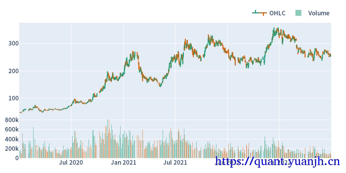
02,行情获取和可视化
a,时间交易参数配置
1 | # Enter your parameters here |
b,获取行情和行情mask
1 | # Download data with time buffer |
origin ohlcv_wbuf size: (978, 5)
Index(['Open', 'High', 'Low', 'Close', 'Volume'], dtype='object')
wobuf_mask ohlcv size: (728, 5)
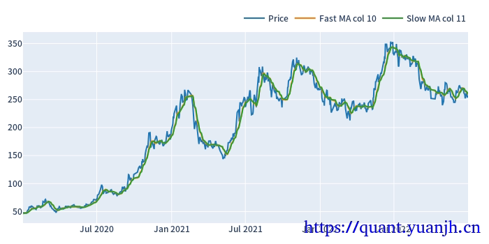
20,网格参数-指标计算和可视化
仅可视化第一列
1 | price=ohlcv_wbuf['Close'] |
(978, 780)
(978, 780)
(728, 780)
(728, 780)
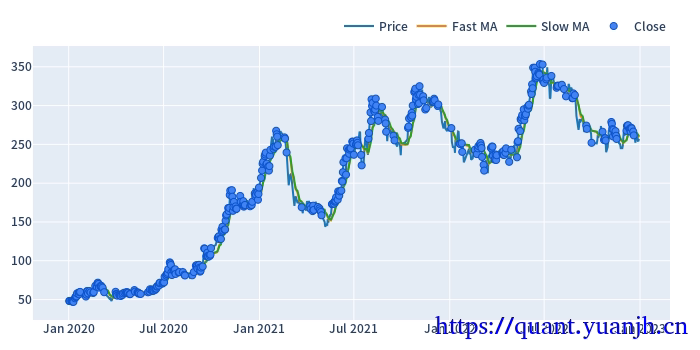
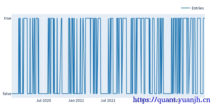
21,网格参数-信号计算和可视化
仅可视化第一列
dmac_size.shape: (728, 780)
dmac_size.iloc[:3,:3]:
fast_window                  10
slow_window                  11    12    13
date
2020-01-02 00:00:00+00:00  True  True  True
2020-01-03 00:00:00+00:00  True  True  True
2020-01-06 00:00:00+00:00  True  True  True
Start                                 2020-01-02 00:00:00+00:00
End                                   2022-12-30 00:00:00+00:00
Period                                                      728
Total                                                423.078205
Rate [%]                                              58.115138
First Index                           2020-01-02 02:00:00+00:00
Last Index                  2022-12-27 06:59:04.615384576+00:00
Norm Avg Index [-1, 1]                                -0.179136
Distance: Min                                               1.0
Distance: Max                                         75.946154
Distance: Mean                                         1.720602
Distance: Std                                          5.889353
Total Partitions                                      14.607692
Partition Rate [%]                                     3.501842
Partition Length: Min                                  3.239744
Partition Length: Max                                 85.138462
Partition Length: Mean                                36.392118
Partition Length: Std                                 27.476308
Partition Distance: Min                                4.425641
Partition Distance: Max                               75.946154
Partition Distance: Mean                              29.174564
Partition Distance: Std                               26.152924
Name: agg_func_mean, dtype: object
22,行情,信号的滑窗处理
注意点:
01,训练集和验证集比例3:1,或者2:1,对应:window_len和set_lens为4:1(或3:1),过大了历史包袱沉重,无法及时响应最新行情,过小了则容易参数跳变,形成类似过拟合效果
a,参数设置和效果预览
代码中
1 | # todo这里是自然日计算的,但后面训练,验证集个数计算都完全正确,哪里应该和预想的不一致 |
1 | # 滚动周期参数设置和大致效果可视化 |
split_kwargs: {'n': 11, 'window_len': 240, 'set_lens': (80,), 'left_to_right': False}
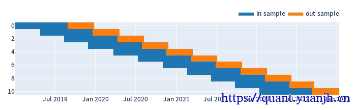
in_price.shape: (160, 11)
out_price.shape: (80, 11)
in_price.index: RangeIndex(start=0, stop=160, step=1)
in_price.columns: Int64Index([0, 1, 2, 3, 4, 5, 6, 7, 8, 9, 10], dtype='int64', name='split_idx')
in_price[0:3]: split_idx     0      1      2      3      4      5       6       7       8       9       10
0          49.17  58.15  51.20  43.39  48.15  97.90  167.98  239.52  202.00  251.77  253.14
1          48.06  56.16  49.50  43.15  49.73  96.55  164.08  225.00  214.11  252.50  266.49
2          50.65  55.36  50.29  43.79  52.25  94.50  168.03  208.99  227.02  246.86  266.08
in_indexes[:5]: [DatetimeIndex(['2019-01-02 00:00:00+00:00', '2019-01-03 00:00:00+00:00', '2019-01-04 00:00:00+00:00', '2019-01-07 00:00:00+00:00', '2019-01-08 00:00:00+00:00', '2019-01-09 00:00:00+00:00', '2019-01-10 00:00:00+00:00', '2019-01-11 00:00:00+00:00', '2019-01-14 00:00:00+00:00', '2019-01-15 00:00:00+00:00',
               ...
               '2019-08-14 00:00:00+00:00', '2019-08-15 00:00:00+00:00', '2019-08-16 00:00:00+00:00', '2019-08-19 00:00:00+00:00', '2019-08-20 00:00:00+00:00', '2019-08-21 00:00:00+00:00', '2019-08-22 00:00:00+00:00', '2019-08-23 00:00:00+00:00', '2019-08-26 00:00:00+00:00', '2019-08-27 00:00:00+00:00'], dtype='datetime64[ns, UTC]', name='split_0', length=160, freq=None), DatetimeIndex(['2019-04-24 00:00:00+00:00', '2019-04-25 00:00:00+00:00', '2019-04-26 00:00:00+00:00', '2019-04-29 00:00:00+00:00', '2019-04-30 00:00:00+00:00', '2019-05-06 00:00:00+00:00', '2019-05-07 00:00:00+00:00', '2019-05-08 00:00:00+00:00', '2019-05-09 00:00:00+00:00', '2019-05-10 00:00:00+00:00',
               ...
               '2019-12-04 00:00:00+00:00', '2019-12-05 00:00:00+00:00', '2019-12-06 00:00:00+00:00', '2019-12-09 00:00:00+00:00', '2019-12-10 00:00:00+00:00', '2019-12-11 00:00:00+00:00', '2019-12-12 00:00:00+00:00', '2019-12-13 00:00:00+00:00', '2019-12-16 00:00:00+00:00', '2019-12-17 00:00:00+00:00'], dtype='datetime64[ns, UTC]', name='split_1', length=160, freq=None), DatetimeIndex(['2019-08-12 00:00:00+00:00', '2019-08-13 00:00:00+00:00', '2019-08-14 00:00:00+00:00', '2019-08-15 00:00:00+00:00', '2019-08-16 00:00:00+00:00', '2019-08-19 00:00:00+00:00', '2019-08-20 00:00:00+00:00', '2019-08-21 00:00:00+00:00', '2019-08-22 00:00:00+00:00', '2019-08-23 00:00:00+00:00',
               ...
               '2020-03-26 00:00:00+00:00', '2020-03-27 00:00:00+00:00', '2020-03-30 00:00:00+00:00', '2020-03-31 00:00:00+00:00', '2020-04-01 00:00:00+00:00', '2020-04-02 00:00:00+00:00', '2020-04-03 00:00:00+00:00', '2020-04-07 00:00:00+00:00', '2020-04-08 00:00:00+00:00', '2020-04-09 00:00:00+00:00'], dtype='datetime64[ns, UTC]', name='split_2', length=160, freq=None)]
b,根据滑窗参数切分行情数据和信号
1 | (in_price, in_indexes), (out_price, out_indexes) = roll_in_and_out_samples(price, **split_kwargs) |
in_price.shape: (160, 11)
out_price.shape: (80, 11)
2019-01-02 00:00:00+00:00
2019-04-24 00:00:00+00:00
DatetimeIndex(['2019-03-25 00:00:00+00:00', '2019-03-26 00:00:00+00:00'], dtype='datetime64[ns, UTC]', name='split_0', freq=None)
###################
in_dmac_size.shape: (160, 8580)
in_dmac_size.iloc[:5,:5]:
split_idx       0
fast_window    10
slow_window    11    12    13    14    15
0            True  True  True  True  True
1            True  True  True  True  True
2            True  True  True  True  True
3            True  True  True  True  True
4            True  True  True  True  True
23,滑窗的收益数据计算
a,持有参数收益
在此区间,基础标的物表现
1 |
|
split_idx
0    0.235446
1   -1.630616
2    0.598889
3    2.647397
4    4.501923
Name: sharpe_ratio, dtype: float64
split_idx
0   -0.929956
1    2.065991
2    4.100300
3    4.801291
4    0.688785
Name: sharpe_ratio, dtype: float64
b,网格参数收益(训练集和验证集)
(8580,)
fast_window  slow_window  split_idx
10           11           0            0.235446
             12           0            0.235446
             13           0            0.235446
             14           0            0.235446
             15           0            0.235446
                                         ...
46           48           10           1.161184
             49           10           1.325572
47           48           10           1.088731
             49           10           1.129224
48           49           10           0.958552
Name: sharpe_ratio, Length: 8580, dtype: float64
(8580,)
fast_window  slow_window  split_idx
10           11           0           -0.703309
             12           0           -0.703309
             13           0           -0.703309
             14           0           -0.929956
             15           0           -0.929956
                                         ...
46           48           10          -0.119443
             49           10           0.516152
47           48           10          -0.119443
             49           10          -0.160922
48           49           10          -0.160922
Name: sharpe_ratio, Length: 8580, dtype: float64
c,训练集上的最佳参数用于验证集
大致思路:
01,获取各split_idx的最佳收益(sharp_radio)的参数组合idxmax,也就是fast_window,slow_window,split_idx,三维索引元组
02,按照split_idx进行聚类,取得各split_idx对应的最佳参数。实际含义就是各滑动窗口的最佳参数
1 | def get_best_index(performance, higher_better=True): |
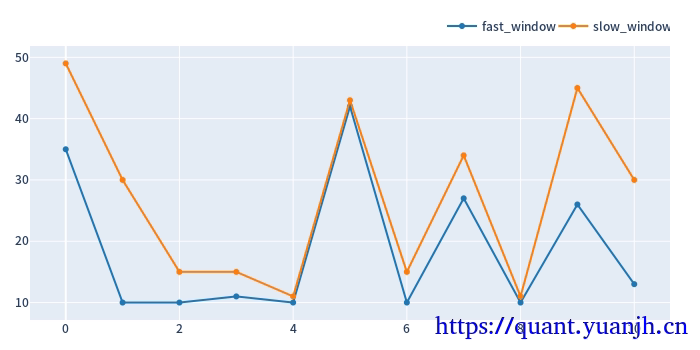
MultiIndex([(35, 49, 0),
            (10, 30, 1),
            (10, 15, 2),
            (11, 15, 3),
            (10, 11, 4)],
           names=['fast_window', 'slow_window', 'split_idx'])
[[35 49]
 [10 30]
 [10 15]
 [11 15]
 [10 11]]
将滚动获取的最佳参数用于验证集,统计收益信息
1 | print('out_dmac_size.shape:',out_dmac_size.shape) |
out_dmac_size.shape: (80, 8580)
in_best_index.shape: (11,)
in_best_index: MultiIndex([(35, 49,  0),
            (10, 30,  1),
            (10, 15,  2),
            (11, 15,  3),
            (10, 11,  4),
            (42, 43,  5),
            (10, 15,  6),
            (27, 34,  7),
            (10, 11,  8),
            (26, 45,  9),
            (13, 30, 10)],
           names=['fast_window', 'slow_window', 'split_idx'])
out_dmac_size.columns: MultiIndex([( 0, 10, 11),
            ( 0, 10, 12),
            ( 0, 10, 13),
            ( 0, 10, 14),
            ( 0, 10, 15),
            ( 0, 10, 16),
            ( 0, 10, 17),
            ( 0, 10, 18),
            ( 0, 10, 19),
            ( 0, 10, 20),
            ...
            (10, 45, 46),
            (10, 45, 47),
            (10, 45, 48),
            (10, 45, 49),
            (10, 46, 47),
            (10, 46, 48),
            (10, 46, 49),
            (10, 47, 48),
            (10, 47, 49),
            (10, 48, 49)],
           names=['split_idx', 'fast_window', 'slow_window'], length=8580)
out_dmac_size.columns.names: ['split_idx', 'fast_window', 'slow_window']
in_best_index.names: ['fast_window', 'slow_window', 'split_idx']
out_dmac_size_reindexed[in_best_index].shape: (80, 11)


    id  col        size  entry_idx  entry_price  entry_fees  exit_idx  exit_price  exit_fees           pnl    return  direction  status  parent_id
0    0    0  199.762836          0    49.934525   24.937656        79       46.85        0.0   -641.111119 -0.064271          0       0          0
1    1    1  222.599259          0    44.811750   24.937656        79       58.80        0.0   3088.836429  0.309656          0       0          1
2    2    2  182.338041          0    54.706425   24.937656        79       88.73        0.0   6178.854345  0.619430          0       0          2
3    3    3  114.462060          0    87.147325   24.937656        79      183.53        0.0  11007.221874  1.103474          0       0          3
4    4    4   59.581957          0   167.417500   24.937656        79      176.88        0.0    538.856616  0.054020          0       0          4
5    5    5   56.155465          0   177.632975   24.937656        79      250.50        0.0   4066.944030  0.407711          0       0          5
6    6    6   39.282222          0   253.933250   24.937656        79      321.74        0.0   2638.662163  0.264526          0       0          6
7    7    7   33.080178         35   301.541975   24.937656        79      240.60        0.0  -2040.909064 -0.204601          0       0          7
8    8    8   41.989226          0   237.562425   24.937656        79      314.89        0.0   3221.987364  0.323004          0       0          8
9    9    9   33.376449          0   298.865300   24.937656        79      274.21        0.0   -847.844011 -0.084996          0       0          9
10  10   10   39.143143         44   254.835500   24.937656        79      266.59        0.0    435.170415  0.043626          0       0         10
fast_window  slow_window  split_idx
35           49           0           -0.929956
10           30           1            2.065991
             15           2            4.100300
11           15           3            4.801291
10           11           4            0.688785
Name: sharpe_ratio, dtype: float64
24,sharp ratio的汇总可视化
1 | cv_results_df = pd.DataFrame({ |
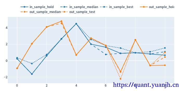
关注点:
蓝色部分
正常排序是(从上到下):点线,实现,线段,
橘色部分
实线对实线
说明测试集和验证集的周期收益情况,二者同时出现0轴同侧较好(同时上涨,同时下跌,保持行情的稳定性or延续性)
线段对线段
二者一方面随着各自颜色的实线趋势变化(受各自实线影响较大),其他应该无必然联系
点线对点线
蓝色点高于橘色点线,蓝色是训练集内最佳,橘色则是训练集得到最优参数用于验证集结果收益,大概率低于验证集。
测试,验证集时间长度差异,引入偏差
由于测试集一般是验证集的2-3倍(或更多),对于单边行情(假如上涨),则(测试集的)实线收益。蓝色线大概率位于橘色线上方。
如果下跌,则相反。蓝色由于时间长,大概率位于橘色下方。
注意:
01,202406,对于当前case,y周取值为sharp ratio夏普比,而非收益率。所以数据点高低并不反映收益率。
所以,以上结论需要稍斟酌,并不完全准确。
25,滚动回测收益可视化
1 | # 验证集:原始价格变动 |
out_price_org shape: (11,)
split_idx
0    0.940574
1    1.315436
2    1.625985
3    2.111239
4    1.059162
dtype: float64
############
out_hold_return shape: (11,)
split_idx
0   -0.064111
1    0.308884
2    0.617885
3    1.100722
4    0.053886
Name: total_return, dtype: float64
############
out_test_return shape: (11,)
fast_window  slow_window  split_idx
35           49           0           -0.064111
10           30           1            0.308884
             15           2            0.617885
11           15           3            1.100722
10           11           4            0.053886
Name: total_return, dtype: float64
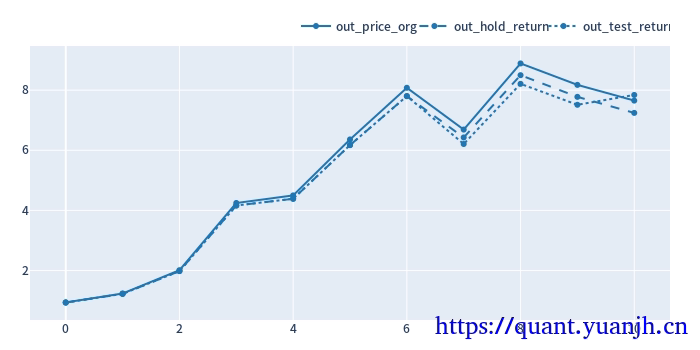
可见,整体结果尚可,上涨幅度基本吃到位,由于单纯依赖技术指标退出,没有止损。所以回撤也是无法避免的。
进一步思考
(非滚动模式)网格参数寻优得到的固定参数,其实是使用未来信息的(未来行情),不符合实际,也就是实际上无法落地。(5月份时,无法知道未来5-10月份,某个参数会取得较好收益)
滚动的网格参数寻优更符合实际,不含未来信息(可落地)。
时间周期越长,基于(非滚动模式)网格参数寻优取得较高收益概率越大,本质上是对历史的拟合。
但是滚动的测试未必,由于其未使用未来信息,如果策略本身无效,则大概率围绕0波动,类似随机。
26,计算正确性验证(略)
a,准备校验数据,数据展示
b,行情->指标 计算正确
0
23
26
22
24
28
c,指标->信号 计算正确
d,信号->交易 计算正确