基于vectorbt的基础唐奇安通道
09dc_01basic:基础方法
09dc_01basicV2:和基础方法等价,不过是基于vectorbt的指标机制的集成的dch指标。
01,基础配置信息
1 | #conda envs:vectorbt_env |
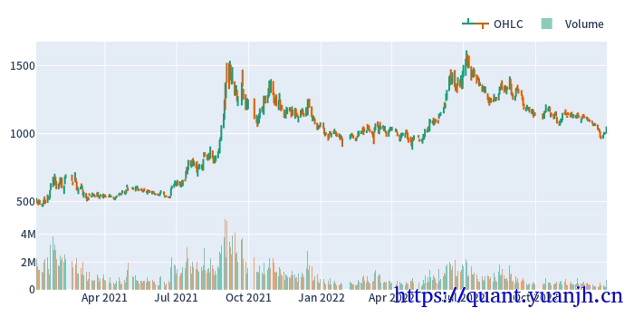
02,行情获取和可视化
a,时间交易参数配置
1 | # Enter your parameters here |
b,获取行情和行情mask
1 | # Download data with time buffer |
origin ohlcv_wbuf size: (1409, 5)
Index(['Open', 'High', 'Low', 'Close', 'Volume'], dtype='object')
wobuf_mask ohlcv size: (485, 5)
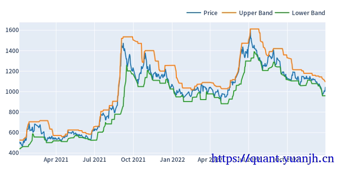
03,指标计算和可视化
1 | # fig.show_svg() |
(1409,)
(1409,)
(485,)
(485,)
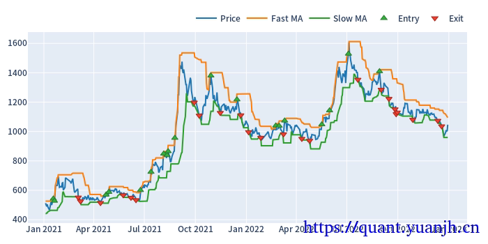
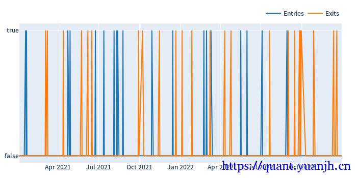
04,信号计算和可视化
1 | # def crossed_above(series1, series2): |
Start                       2021-01-04 00:00:00+00:00
End                         2022-12-30 00:00:00+00:00
Period                                            485
Total                                              19
Rate [%]                                     3.917526
Total Overlapping                                   0
Overlapping Rate [%]                              0.0
First Index                 2021-01-18 00:00:00+00:00
Last Index                  2022-08-29 00:00:00+00:00
Norm Avg Index [-1, 1]                       -0.19552
Distance -> Other: Min                            3.0
Distance -> Other: Max                           67.0
Distance -> Other: Mean                     25.315789
Distance -> Other: Std                       17.34952
Total Partitions                                   19
Partition Rate [%]                              100.0
Partition Length: Min                             1.0
Partition Length: Max                             1.0
Partition Length: Mean                            1.0
Partition Length: Std                             0.0
Partition Distance: Min                           2.0
Partition Distance: Max                          61.0
Partition Distance: Mean                    21.722222
Partition Distance: Std                     18.549792
dtype: object
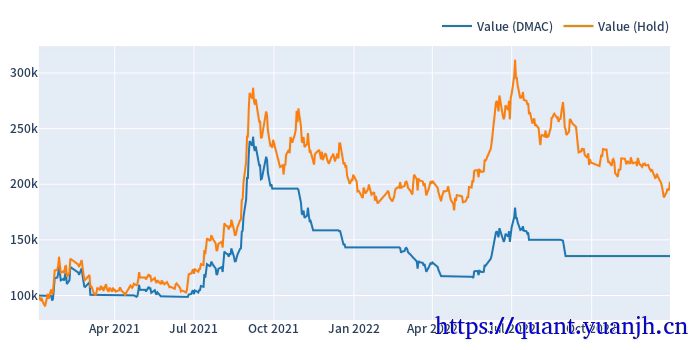
05,交易统计
a,基准比对
1 | dmac_pf = vbt.Portfolio.from_signals(ohlcv['Close'], dc_entries, dc_exits) |
Start                         2021-01-04 00:00:00+00:00
End                           2022-12-30 00:00:00+00:00
Period                                              485
Start Value                                    100000.0
End Value                                 135478.738311
Total Return [%]                              35.478738
Benchmark Return [%]                         104.325952
Max Gross Exposure [%]                            100.0
Total Fees Paid                             6084.898884
Max Drawdown [%]                               52.33349
Max Drawdown Duration                             318.0
Total Trades                                          9
Total Closed Trades                                   9
Total Open Trades                                     0
Open Trade PnL                                      0.0
Win Rate [%]                                  33.333333
Best Trade [%]                                97.749209
Worst Trade [%]                              -19.171936
Avg Winning Trade [%]                         42.098525
Avg Losing Trade [%]                          -9.811332
Avg Winning Trade Duration                         47.0
Avg Losing Trade Duration                          11.0
Profit Factor                                  1.374907
Expectancy                                  3942.082035
dtype: object
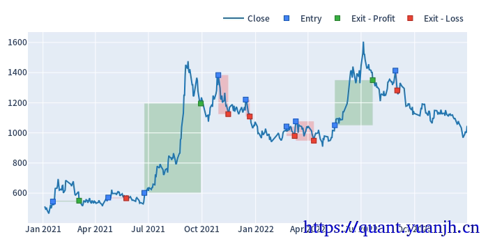
b,交易详情和可视化
1 | # Plot trades |
   id  col        size  entry_idx  entry_price  entry_fees  exit_idx   exit_price   exit_fees           pnl    return  direction  status  parent_id
0   0    0  183.350720         10   544.042715  249.376559        38   550.239953  252.217228    634.674170  0.006363          0       1          0
1   1    0  175.831773         73   570.907710  250.959287        91   565.963545  248.785934  -1369.086519 -0.013639          0       1          1
2   2    0  164.485565        113   601.986212  247.545106       180  1194.915225  491.365766  96789.353009  0.977492          0       1          2
3   3    0  141.336528        197  1383.690600  488.915064       208  1124.681250  397.396358 -37493.793739 -0.191719          0       1          3
4   4    0  129.545854        230  1220.924700  395.414331       235  1108.431975  358.981916 -15327.362345 -0.096907          0       1          4